Architecture of the visual cortex
Compared to the external geniculate body (ECC) and the retina, the primary visual cortex, or striate cortex, is a much more complex structure. As we have already seen, a sharp increase in the structural complexity of brain regions is accompanied by a similar complication of physiological organization. In the striate cortex we find a greater diversity of functional cell types. Neurons in the striate cortex respond to more complex stimuli, i.e. stimuli with a large number of parameters, and these parameters must be quite specific. While in the study of retinal cells and NKTs we only had to change the location and size of the stimulus in the form of a simple spot, now we are suddenly faced with the need to take into account such parameters as the orientation of the line, the direction of movement, the length of the line and its curvature, as well as the choice of the eye to which the stimulus is applied. What relationship, if any, exists between these parameters and the structural organization of the cortex? In order to approach this question, it is first necessary to say something about the structure of the striate cortex.
Anatomy of the visual cortex
The cortex is a layer of nervous tissue about 2 mm thick that almost completely covers the cerebral hemispheres. The surface area of the human cortex is more than a square foot (about 900 cm2). The total area of the cortex in macaques is approximately 10 times less than in humans. It has been known for more than a century that the cerebral cortex is divided into many different cortical fields. Among all these fields, the first was able to isolate the zone of the primary visual cortex, which in cross sections looks layered or striped (hence its long-standing name - striate cortex: Latin stria - stripe). There was a time when all the aspirations of neuromorphologists were to identify as many cortical fields as possible on the basis of sometimes very subtle histological differences. In one of the accepted systems of such classification, the striate cortex was assigned the number 17. According to one of the newest estimates (D. van Essen, California Institute of Technology), in macaques the primary visual cortex occupies about 1200 mm2 (a little less than one third of a credit card); this is approximately 15% of the total area of the cortex, i.e. quite a significant part of it.
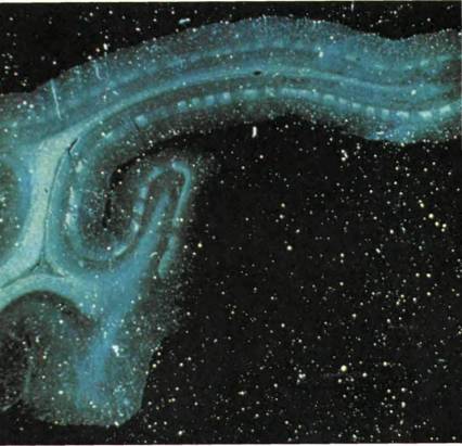
Rice. 60. This section shows columns of ocular dominance in the cortex of the left hemisphere of the macaque brain. The cut is made perpendicular to the surface of the bark in the direction from left to right. As we trace the surface of the bark from left to right (see top of photo), we see that it forms a curve and a deep fold running from right to left. The radioactive amino acid, injected into the animal's left eye, was transported through the tubing into layer 4C of the cortex and concentrated in many separate areas, each half a millimeter thick, that stand out as bright stripes against a generally dark background. (The solid light leaf in the middle is a white substance consisting of fibers from the geniculate body.)
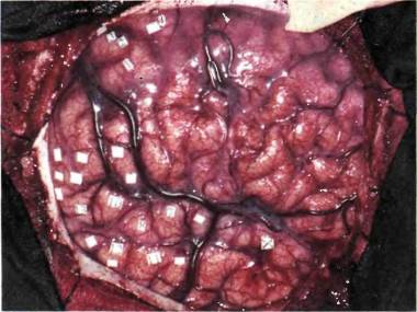
Rice. 61. A large portion of the right cerebral cortex is visible here, exposed under local anesthesia for neurosurgery for epilepsy. The patient was fully conscious. The operation was performed by surgeon Dr. W. Feindel at the Montreal Neurological Institute. The area of the scalp was turned away and the corresponding piece of the skull was removed (temporarily, until the end of the operation). The image shows grooves, convolutions, large purple veins and smaller (red) arteries. The overall pinkish tint of the exposed part of the brain is due to the presence of a fine network of branches of these vessels. The lower third of the exposed area is the temporal lobe. Above the horizontally running large veins are parts of the parietal lobe (left) and frontal lobe (right). At the very left edge you can see a strip of the occipital lobe. The operation was carried out to treat a certain form of epilepsy and involved removing the affected part of the brain. Such an operation is allowed only if it cannot lead to disruption of voluntary movements or speech. To avoid this, the neurosurgeon uses electrical stimulation to identify areas associated with speech, movement and sensitivity, finding out what motor effects, sensations in different parts of the body and speech disorders occur. It is clear that such tests would be impossible if the patient were not conscious. The places where irritation was performed are marked with pieces of sterile paper with numbers. With irritation, for example, the following results were noted: 1) a tingling sensation in the thumb of the left hand; 2) tingling in the ring finger of the left hand; 3) tingling in the ring and middle fingers of the left hand; 4) bending the fingers of the left hand and wrist. When areas numbered 8 and 13 were irritated, more complex phenomena arose, similar to memory images, which happens in some patients with epilepsy when the temporal lobe is irritated.
In Fig. 62 shows a photograph of a macaque brain (rear view). The skull was removed, and the brain was perfused with a dilute solution of formaldehyde for preservation purposes, which gave it a yellow color. Usually, on the surface of the cortex, a network of blood vessels is striking, but here they are in a collapsed state and therefore invisible. This photograph shows mainly the surface of the occipital lobe of the cortex, i.e. that area that is directly related to vision and includes not only the striate cortex, but also one or two dozen (and maybe more) prestriate zones To fit a 0.5-mm-thick piece of neural tissue, the size of a large index card, into a box the size of a macaque skull, one would have to crumple the piece, much like we crumple up a piece of paper before throwing it in the trash. As a result of similar compression, gaps are formed in the cerebral cortex, or furrows, between which there are convex sections called convolutions.
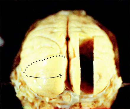
Rice. 62. Brain of a macaque (back view). Shown is the occipital lobe and the part of the striate cortex that extends to the surface of this lobe (below the dotted line).
The area in the photograph that lies behind (below) the dotted line is the open, visible part of the striate cortex. Although the striate cortex occupies most of the surface of the occipital lobe, in the photo we can see only part of it (0.3–0.5 of the total area); the rest is hidden in the furrow.
The striate cortex (field 17) has many output fibers, a significant part of which goes to the next cortical area - visual field 2, often also called area 18, since it is adjacent to area 17. Area 18 is a strip of bark approximately 6–8 mm wide, almost completely surrounding area 17. In the photo (Fig. 62) only part of area 18 can be seen, located above the dotted line, which corresponds to the border between areas 17 and 18; Most of field 18 goes down into a deep furrow located just in front of the dotted line. Field 17 is ordered, point to point, projected onto field 18, and the latter in turn forms projections in at least three occipital zones, each the size of a postmark. These areas are known as area MT (short for medialis temporalis) and visual areas 3 and 4 (often referred to as V3 and V4). As a rule, each cortical zone has projections to several other zones located at a higher level. In addition, for each zone of the cortex, you can find a reverse projection - to the zone or zones from which the input fibers come. And as if striving for even greater complexity, each of these zones forms projections in deep structures of the brain, for example, in the superior colliculus and in various parts of the thalamus (a complex cellular structure the size of a golf ball, a small part of which is the NKT). And all these visual areas receive input signals from different parts of the thalamus - just as the NKT projects to the primary visual cortex, so different areas of the thalamus form projections in other cortical areas.
In the same photograph, the letter X indicates that portion of field 17 that receives input signals from the central fovea of both retinas. If you move along the left hemisphere from point X in the direction indicated by the arrow, then in the field of view this will correspond to the horizontal movement of the object from the fixation point. If, having left point X again, we move straight along the boundary between fields 17 and 18, then this will correspond to the movement of the object downwards from the fixation point, and movement in the opposite direction will correspond to the movement of the object upwards. The arrow itself in the field of view corresponds to a horizontal line about 6° long. Areas of the visual field located further than 9° from the center of gaze are mapped to that part of field 17 that lies in the cortical fold under the outer surface of the brain, parallel to it.
To see what the cortex looks like in cross section, we cut out a section of the visual cortex from the right half of the brain shown in Fig. 62. The resulting section was treated with cresyl violet, which stains the cell bodies of neurons blue, but does not stain axons and dendrites. In this micrograph taken at low magnification, individual cells cannot be distinguished, but dark layers of densely packed cells can be seen and lighter layers with many fewer cells. Under the outer surface of the bark, a complex structure of folds is visible, resembling a mushroom in shape. In reality, this structure and the superficial part of the cortex merge into each other without interruption. The light-colored space is a white substance that fills the areas between the outer parts of the cortex and its deeper folds. White matter consists mainly of myelinated nerve fibers that are not stained with dye. The part of the cortex containing the bodies of nerve cells, their axons and dendrites, as well as synapses, forms gray matter.
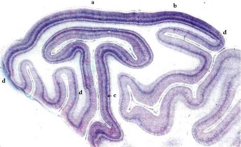
Rice. 63. Section of the occipital lobe of the brain (from the area shown in Fig. 62): it corresponds to the left wall of the groove cut in the right hemisphere). Letter а the point lying at the level of the X–> arrow is marked. Nissl staining allows you to see only the cell bodies, but they are so small that they look like dots. The darker areas above and the mushroom fold below correspond to the striate cortex. Three letters d the boundaries between fields 17 and 18 are indicated.
In terms of the complexity of its layered structure, field 17 surpasses all other zones of the cortex. This difference can be seen even at low magnification (Fig. 63), if you compare field 17 and the neighboring area on the right - field 18 (the border between them is marked with the letter г). One more detail: if you compare in Fig. 63 regions a, b и V, where different parts of the visual field are projected (their distances from the point of fixation are <5, 6 and 80–90 degrees, respectively), we will not notice a significant difference in either the thickness of the cortex or its layered structure. As it turns out, this homogeneity is important. I will return to this issue later in this chapter.
Layers of the visual cortex
In Fig. 64 shows a small section of field 17 at a higher magnification. Here it is already possible to distinguish the bodies of individual cells in the form of points and get some idea of their size, number and distribution. The visible pattern of layers is partly determined by the intensity of cell staining and partly by the density of their packing. Layers 4C and 6 are the densest and darkest. In layers 1, 4B and 5, the cells are most loosely located. Layer 1 barely contains a single nerve cell, but there are many axons, dendrites, and synapses. In order to show that different layers contain different types of cells, it is necessary to apply some version of the technique invented in 1900 by C. Golgi. Golgi staining reveals only a few cells, but in sections the entire cell is visible, including its axon and dendrites. The two main classes of cortical cells are pyramidal cells, found in all layers of the cortex except layers 1 and 4, and stellate cells, found in all layers. Examples of pyramidal and stellate cells are shown in Fig. 4. A typical distribution of pyramidal cells in the cortex is shown in Ramon y Cajal’s drawing in his book “Histology” (Fig. 65); This depicts only a small fraction of all pyramidal cells present in this area, probably about 1 percent.
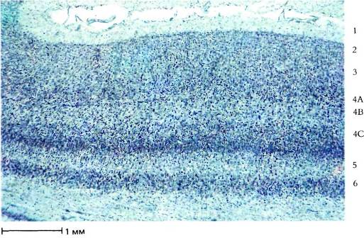
Rice. 64. Transverse section of the striate cortex at higher magnification. Cells arranged in layers are visible. Layers 2 and 3 cannot be separated from each other; Layer 4A is very thin. The thick, light layer at the bottom is a white substance.
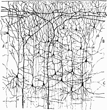
Rice. 65. Golgi-stained section of layers 1, 2 and 3 of the visual cortex of an infant several days old. The black triangles are the cell bodies from which arise apical dendrites that rise upward and branch in layer 1, basal dendrites that extend laterally, and one thin axon that runs straight down.
Fibers coming from the NKT come to the cortex from the white matter of the brain. Passing in a diagonal direction, most of the fibers reach layer 4C, branch repeatedly and finally reach their final destination, forming synapses with stellate cells, which mainly fill this layer. Axons emerging from the two ventral (magnocellular) layers of the NKT terminate in the upper half of layer 4C, called sublayer 4C?, and those emerging from the four dorsal (parvocellular) layers of the NKT terminate in the lower half of layer 4C (sublayer 4C?). As can be seen from the diagram in Fig. 66, these two sublayers form different projections in the upper layers - 4C? sends signals to 4B, but 4C? - into layers 2 and 3. The latter, in turn, also differ in their projections. The marked difference in the neural pathways emerging from the two groups of tubular layers is one of many reasons to believe that two different systems are associated with these pathways. Most pyramidal cells in layers 2, 3, 4B, 5, and 6 have axons emerging from the cortex, but these axons have branches (collaterals) that form local connections and thus help distribute information throughout the cortex.
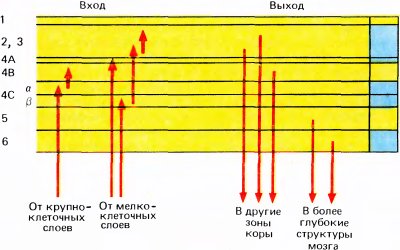
Rice. 66. Major pathways from HKT to the striate cortex and from the striate cortex to other brain areas. On the right side of the diagram, zones with the highest Nissl color density are marked (for comparison with Fig. 64).
The cortical layers differ not only in their inputs and internal connections, but also in the addresses of the structures to which they are projected. All of them, except layers 1, 4A and 4C, have output fibers extending beyond the cortex. The upper layers 2 and 3, as well as layer 4B, send signals mainly to other areas of the cortex, while the lower layers project to subcortical structures: from layer 5, output fibers go to the midbrain, to the superior colliculus, and from layer 6, fibers are sent back to the NKT. Although it has been known for almost a century that the output fibers of the NKT go mainly to cortical layer 4, we knew nothing about the differences between the outputs of different layers of the cortex until Japanese researcher K. Toyama first discovered these differences in physiological experiments in 1969. Since then, these data have been repeatedly confirmed by morphological methods.
Ramon y Cajal was the first to realize how short the internal connections in the cortex are. As already mentioned, the most numerous connections go up and down, closely uniting different layers. Diagonal and lateral (horizontal) bonds are typically 1 to 2 mm in length, although some bonds can be traced over a distance of 4 to 5 mm. This limitation of the “horizontal” transmission of information in the cortex leads to important consequences. If the inputs are organized according to a topographical principle (in the case of the visual system, in accordance with the position of the displayed point on the retina or in the visual field), then the same principle must be preserved in the organization of outputs. Whatever functions the cortex performs, the analysis performed must be local. Information about any small area of the visual field enters some small area of the cortex, where it undergoes transformation, analysis, processing (call it whatever you want) and is transferred somewhere for further processing, regardless of what happens to the information about the neighboring area. Thus, the image of the visual scene is analyzed as if in a mosaic. Therefore, the primary visual cortex cannot be the place where entire objects are recognized, perceived, or otherwise processed, such as boats, hats, faces, i.e. cannot be the substrate of “perception” processes. Of course, such a general conclusion is hardly legitimate to draw on the basis of anatomical data alone: after all, information could be transmitted over long distances along the cortex and according to the relay race principle, with separate stages of one millimeter each. However, by recording the activity of cells during simultaneous stimulation of the retina, it can be shown that this is not the case: it turns out that all cells in a given small area have small receptive fields and that neighboring cells always have receptive fields located in almost the same place. There is no physiological evidence to indicate that any cell in the primary visual cortex of a monkey is connected to any other cell at a distance greater than 2–3 millimeters.
Clinical neurological data have long indicated the “mosaic” nature of information processing. After small strokes, tumors, or injuries to the primary visual cortex, complete blindness can occur in small, well-defined areas of the visual field. At the same time, normal vision is maintained in all other areas. If every cell were connected in some way to every other cell, then some general, non-local impairment of vision would be expected instead. Moving somewhat away from our topic, it should be noted that patients with such lesions may not be aware of the presence of a visual field defect, especially in cases where the part of the cortex where the projection of the central fovea of the retina is located is not affected, i.e. points of gaze fixation. In any case, such patients do not see completely black or completely gray islands, or any other defects in their field of vision. Even if the entire occipital lobe on one side is destroyed and a person sees nothing in the opposite half of the visual field, he does not have the impression that the visual world is closed from him on this side. I myself sometimes have migraine attacks (fortunately without headaches) with short-term blindness, often in a large part of one of the hemifields of vision. If you ask What exactly I see in this area, I can only say that I see literally nothing - neither white, nor gray, nor black, just nothing.
Another curious feature observed in patients with an island of local blindness, or scotoma, is a phenomenon known as “filling in.” If a person with a scotoma looks at a line passing through the defective part of the visual field, he will not notice any break - the line appears completely continuous. A similar phenomenon can be demonstrated by taking advantage of the fact that the normal eye also has a blind spot. This is where the optic nerve exits the eye. The blind spot is an oval area about two millimeters in size, where there are no rods or cones. You can find a blind spot using a small paper disk - the method is so simple that it is accessible to everyone. First, close one eye, for example the left one. Keeping it closed, fixate with your other eye some small object in the room. Now take a paper disk in your hand and extend your hand to its full length, placing it exactly on the line connecting the eye to the object. Then slowly move your hand to the right exactly horizontally (the presence of a dark background makes the experiment easier). The paper disk will disappear approximately at the moment when its displacement reaches 18°. Now if you take some kind of rod and place it so that it intersects the blind spot, then it will look like a complete object without any breaks. The area occupied by a blind spot is similar to a scotoma - you will not notice its existence until you do the experiment described above. You don't see black or gray or anything else here, you just don't see anything.
Similarly, if you look at a large sheet of white paper, only those cells in the cortex whose receptive fields fall on the edge of the sheet will fire (since cortical cells tend to ignore evenly distributed light). In this case, the cessation of activity of cells whose receptive fields lie entirely within the sheet of paper should lead to the disappearance of brightness differences in this area of the visual field. The island of blindness in this case should not be visible - and it is not visible. We cannot see our blind spot in the form of a black hole in the sheet of white paper we are looking at. The padding phenomenon demonstrated by the paper experiment should convince everyone that we cannot understand how the brain actually works based on intuitions alone.
Cortical architecture
Now we can return to the original question: how are the physiological properties of cortical cells and their structural organization related to each other? We can sharpen this question even further: knowing that cortical cells can differ in the position of their receptive fields, "complexity", preferred stimulus orientation, ocular dominance, in the optimal direction of movement of the stimulus and in the optimal length of the stimulus line, is it reasonable to expect that neighboring cells are similar in some or even all of these parameters? Or are cells with different properties simply scattered randomly throughout the cortex, without any connection with their physiological properties?
Studying the anatomy of the cortex with the naked eye or under a microscope will not help much. In cross sections, clear differences can be seen between the individual layers of the cortex. However, if we trace the same layer along its length in a cross section or study sections of one layer made parallel to the boundary of the layers, we will see only gray homogeneous material. Although such homogeneity may indicate a random distribution of cells, we know that with respect to at least one variable, the cells are arranged in a very orderly manner. We are talking about a natural correspondence between the distribution of cells in the striate cortex and the position of their receptive fields on the retina, i.e. that neighboring cortical cells should have receptive fields located close to each other in the visual field. This is precisely the picture that emerges in experiments. In two cells lying nearby in the cortex, the receptive fields usually even overlap over most of their area. However, these fields do not overlap each other exactly. If the microelectrode is moved along the cortex from cell to cell, the positions of the corresponding receptive fields are shifted in a direction that can be predicted by knowing the topography of the retinal display in the cortex. No one would have doubted this result even 50 years ago, having data on the connections of the NKT with the cortex and on cases of local blindness after strokes. But what about the other parameters—ocular dominance, “complexity,” orientation of adequate stimuli, and others?
It took several years to learn how to reliably stimulate cortical cells and record their responses; As a result, it became possible to describe the reactions not only of individual cells, but also of relatively large groups of neurons. It started with the fact that we accidentally managed to simultaneously record the responses of two or more cells (an example of such a recording was shown in Fig. 59). It is not difficult to write down the answer of two neighboring cells. In those experiments where we determined a cell's preferred stimulus, we almost always used an extracellular lead, placing the tip of the microelectrode next to the cell; in this case, it was not changes in the membrane potential that were recorded, but currents associated with the impulses. It often turned out that we were recording the reactions of not one, but several cells at the same time - say, in the case when the tip of the microelectrode stopped halfway between two neuron bodies. The pulse discharges of single cells with such a lead are almost identical, but the magnitude and shape of the pulses depend on the distance and on the relative position of the cells, so that the discharges taken simultaneously from two cells usually turn out to be different, and therefore they can be easily distinguished. By performing this kind of derivation from two cells, we were able to clearly see how neighboring cells differ and in what ways they are the same.
In one of the first such leads, two cortical cells were discovered that responded to the opposite movements of a hand that was waved in front of the animal. In this case, two cells lying side by side gave different (essentially opposite) responses to the movement of the stimulus. In other respects, however, these cells almost certainly exhibited similar properties. If I had already been prepared to study orientation selectivity in 1956, I would very likely have found that both preferred orientations were close to vertical, since these cells responded well to horizontal movements of the stimulus. The fact that they both responded to the back-and-forth movement of the hand means that the positions of the receptive fields of these cells approximately coincided. If I examined these neurons for ocular dominance, then most likely this parameter would also be the same.
Already in the first recordings of the activity of cortical neurons, we were struck by how often two cells whose responses can be recorded simultaneously are identical in ocular dominance, complexity and, most surprisingly, in optimal stimulus orientation. Such coincidences, which are unlikely to be random, suggest that cells with the same properties are grouped together. The possibility of such a grouping interested us greatly, and as soon as this assumption was confirmed, we began to find out what the size and shape of these groups were.
Cortex research
Using microelectrodes, only individual points of the cortex can be examined. To get an idea of the three-dimensional organization of the brain, you have to slowly immerse the electrode in depth, stop it from time to time to record the activity of one cell (or perhaps two or three cells), mark the depth readings on a special scale, and then repeat all over again. Sooner or later, the tip of the microelectrode will pass through the entire cortex, and then the electrode can be removed and reinserted somewhere else. After the experiment is completed, a section is made, stained, and examined under a microscope to determine the position of each of the nerve cells whose activity was recorded. In one experiment lasting about 24 hours, it is usually possible to make two or three penetrations of approximately 4–5 millimeters each. In one pass, responses from approximately 200 cells can be observed.
The microelectrode is so thin that it is barely possible to detect a trace of its passage under a microscope, so there is no reason to think that when passing through a microelectrode, many cells will be damaged and this could affect the reactions of nearby neurons. Initially, we had difficulty finding the trace of the microelectrode on the histological section, let alone determining the position of the electrode tip, and this made it difficult to assess the position of the cells whose activity was recorded. This difficulty was overcome when it was discovered that passing a weak current through a microelectrode leads to the destruction of cells in the immediate vicinity of the tip of the microelectrode, and this zone of destruction is clearly visible in histological sections. Fortunately, the microelectrode itself is not damaged when current is passed through. Therefore, during one penetration, the current is passed 3–4 times, while noting the depth of immersion of the microelectrode, and since the depth is also noted when recording the activity of cells, the position of each of them can be assessed. Of course, when exposed to current, a few cells near the tip of the microelectrode die, but not so many of them that the work of more distant neurons could be disrupted. In order not to distort the responses of cells lying in front of the microelectrode, its tip is moved forward a little, cell activity is recorded, and then the tip is pulled back and then a current is passed.
Variations in difficulty
As would be expected, cells in the input cortical layer—layer 4—exhibit simpler behavior than cells in the output layer. We have already noted in this chapter that in the monkey, cells in layer 4C?, which receives fibers from the four upper (parvocellular) layers of the NKT, apparently do not have selectivity for stimulus orientation and behave like cells that have round receptive fields with a center and a periphery. In layer 4C?, which has inputs from two ventral (magnocellular) layers of the NKT, some cells have round fields with a center and periphery, and all the rest, apparently, are characterized by simple receptive fields and orientation sensitivity. If we move to the next level—the layers above and below layer 4C—the vast majority of cells are complex. Line end responding cells make up about 20 percent in layers 2 and 3 and are rare in other layers. Thus, in general, there is a clear correlation between the complexity of cells and their position in the visual pathway, which can be estimated by the number of synaptic switches to a given location.
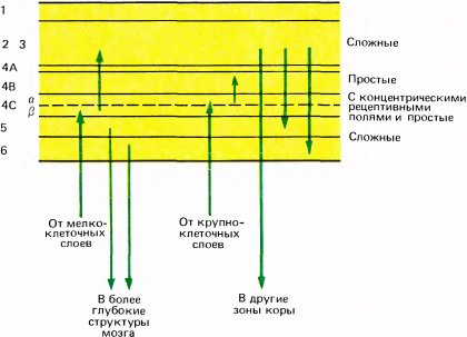
Rice. 67. Approximate diagram of the placement of cells of physiologically different types in different layers of the striate cortex.
The claim that most cells above and below layer 4 are complex overlooks important differences between layers: complex cells here are far from identical. Of course, they all have one common property characteristic of complex cells - they respond to a moving line of optimal orientation throughout the receptive field, regardless of the specific position of the stimulus. However, they differ from each other in other properties. Four subtypes of cells can be distinguished, which are mainly contained in different layers. The majority of complex cells in layers 2 and 3 respond better the longer the stimulus line (this manifests the property summation along length). However, the response of such cells becomes weaker when the stimulus length exceeds a certain critical value (if this complex cell belongs to neurons that respond to the ends of lines). As for the cells of layer 5, for them short lines, occupying only a small fraction of the receptive field in length, are almost as effective as long ones; the receptive fields of these cells are much larger than those of cells in layers 2 and 3. On the contrary, cells in layer 6 respond better the longer the line with the optimal orientation is (their response begins to deteriorate only when the line takes up the entire length of the receptive field, which is several times larger than its width, i.e. the receptive field is long and narrow). It can be concluded that axons emerging from layers 5 and 6 and from layers 2 and 3 and going to different parts of the brain (to the superior colliculus, to the NKT, to other visual fields) should serve to transmit different types of visual information.
To summarize, we can say that when moving from layer to layer, more important differences in cell behavior are revealed than, say, differences in the optimal orientation of the stimulus or in the nature of ocular dominance. The most noticeable differences between cells of different cortical layers concern the complexity of their reactions; this reflects the simple anatomical fact that some layers are located closer to the entrance to the cortex than others.
Columns of eye dominance
Groups of cells in the striate cortex with different ocular dominance were discovered first, since they are quite large. Many methods have been developed for studying such groups, so they are now the best studied. Already at the very beginning of studies on the cortex of monkeys, it became obvious that whenever a microelectrode enters the cortex perpendicular to its surface, it encounters one after another cells that respond better to stimulation of the same eye (this is shown in Fig. 68). If the microelectrode is removed and inserted in another place a few millimeters from the previous one, then again for all the cells encountered, one eye will be dominant - the same as before, or the other. In layer 4C, which has inputs directly from the tubing, the dominance of one eye no longer becomes relative, but absolute, monopoly. In the same layers that are located above and below and, therefore, are located further in the chain of synaptic switchings, more than half of all cells can be excited by the non-dominant eye. We call such cells binocular.
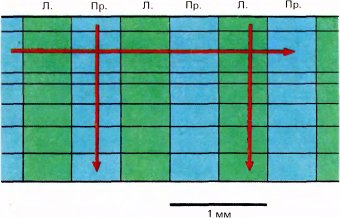
Rice. 68. Ocular dominance remains unchanged with vertical advancement of the microelectrode in the striate cortex. If the electrode moves parallel to the surface of the cortex, then zones with different ocular dominance alternate, and each pair of such zones occupies about 1 mm.
If, instead of moving the electrode perpendicular to the surface of the cortex, we inserted it at an angle, as close as possible to a line parallel to the surface, then cells with different ocular dominance alternated - first one eye was dominant, then the other. The full cycle of this shift corresponded to approximately one millimeter. Obviously, if one could see the structure of the cortex from above, it would appear as a mosaic composed of alternating zones with dominance of the right and left eyes.
The reason for this alternation became clear when a new staining method was developed that made it possible to trace the branching of individual axons coming from the NKT and the distribution of their endings in the cortex. The branching of one axon is such that its thousands of terminal synapses form in layer 4C two or three clusters 0.5 mm wide, separated by intervals of about 0.5 mm, as shown in Fig. 69. Since NKT cells are monocular, each individual axon is ultimately connected to either the right or left eye. Let us assume that the axon shown in Fig. 69 on the left, refers to fibers from the left eye; in this case, each fiber connected to the left eye entering the same area of the cortex will branch in the same clusters of endings, each 0.5 mm in size. The spaces between these clusters, also 0.5 mm in size, will be occupied by the terminal branches of fibers from the right eye. This special type of distribution of axons from the NKT in layer 4C immediately explains the strict monocularity of the cells in this layer.
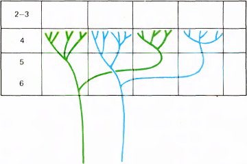
Rice. 69. Each axon from HKT first passes through the lower layers in the striate cortex, branches successively and then terminates in layer 4C. Here it forms clusters of synaptic endings 0.5 mm wide, separated from each other by gaps of the same width. All fibers from one eye are grouped in the same areas. In the spaces between these areas, fibers from the other eye are grouped. The branching area of one fiber from the magnocellular layer of HKT can be from 2 to 3 mm (the endings are in layer 4C?). The fiber from the parvocellular layer of HKT branches in a more limited area (in layer 4C?), usually occupying only one or two columns.
In order to selectively dye one and only one fiber, a new method was required and was proposed in the late 1970s. This method is based on the use of axonal transport, a process by which various materials (proteins or even larger particles) are continuously transported in both directions within the axon. Some of them are transported at a speed of several centimeters per hour, others - several millimeters per day. To stain a single axon, a substance is introduced using a micropipette into it, which is known to be carried along the axon and stain it, but does not affect the structure of the cell. Currently, the enzyme most often used is horseradish peroxidase. This enzyme travels along the axon in both directions and catalyzes a chemical reaction, the product of which very effectively stains the cell. Since the enzyme serves as a catalyst, tiny amounts are sufficient to produce intense color. It is also important that there is no enzyme with similar properties in the nervous tissue itself: this eliminates the possibility of unwanted background coloring.
The fact that the cortex is divided into columns of ocular dominance extending from the surface of the brain all the way to the white matter supported the morphological evidence that groups of cells in layer 4C serve as the main sites for the transmission of visual information to the cellular layers lying above and below this layer. The presence of a certain number of horizontal and diagonal connections about a millimeter long, running in all directions, should lead to some blurring of clear zones of dominance of the right or left eye in the layers located above and below layer 4C (Fig. 70). Therefore, one would expect that a cell located directly above the center of the left eye dominance zone in layer 4 would be clearly better responsive to stimulation of that eye (and perhaps even fully controlled by it), whereas a cell located closer to the boundary between areas of different ocular dominance might be binocular without any dominance of one eye. Indeed, with horizontal movement of the electrode in the upper layer of the cortex or in layers 5 or 6, gradual changes in ocular dominance are observed: first, there will be cells that are much more strongly activated by one eye, then cells in which this asymmetry is less pronounced, then cells with equal dependence on both eyes, after which the influence of the other eye will begin to increase. Such smooth transitions contrast sharply with the sudden change in ocular dominance that we observe when the electrode moves along layer 4C (Fig. 71).
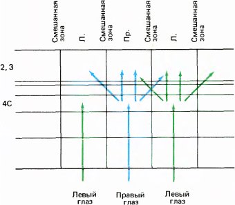
Rice. 70. Due to the presence of horizontal and diagonal connections above layer 4, the ocular dominance columns overlap and their boundaries are blurred.
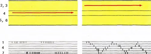
Rice. 71. In contrast to the clear boundaries between the columns of ocular dominance in layer 4 of the cortex, the boundaries of the columns in the upper (2 and 3) and lower (5 and 6) layers of the cortex are blurred. The arrows indicate the direction of microelectrode advancement in layer 4 (top left) and in layer 2 or 3 (top right). Below is the ocular dominance of cells whose responses were recorded in one passage of the microelectrode. In layer 4, sharp transitions are visible from group 1 (only the contralateral eye is affected) to group 7 (only the ipsilateral eye is affected). In other layers there are many binocular cells, and ocular dominance periodically changes, passing through intermediate levels (numbers 1, 4 and 7 indicate categories of cells according to ocular dominance).
When viewed from the side, the two sets of cells in layer 4C appear as alternating patches. However, we wanted to know what the distribution of these areas would look like when looking at the surface of the cortex from above. Let us assume that they are marked on the surface of the cortex in black or white. From a topological point of view, these areas can be distributed in several different ways: in a checkerboard pattern, in the form of alternating black and white stripes, in the form of black spots on a white background, or any combination of these patterns. In Fig. Figure 72 shows three possible options for such a distribution. Solving a given problem using microelectrodes alone means using one-dimensional means to decipher an unknown three-dimensional structure. This is a hopeless task - like trying to cut the grass on your lawn with nail scissors. Faced with such difficulties, many would prefer to switch to a completely different type of activity - to engage in, say, agriculture or law. (In the early 1960s, when Thorsten Wiesel and I were more patient and determined than we are now, we actually tried to figure out the topography of ocular dominance using microelectrodes, and we even managed to get some results. Figuratively speaking, I actually tried to cut the grass lawn with scissors in those days, since we could not afford to buy a lawn mower. We were poorer then than today's graduate students, however were probably more persistent.)
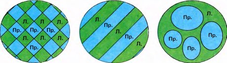
Rice. 72. Shown here are three possible ways of dividing a surface into two types of areas—checkerboard, stripe, and island. In this case, we are talking about the surface of the cortex and the areas of dominance of the right or left eye.
Fortunately, very effective methods for neuromorphological research have been invented in the last ten years, and now the task we have posed has already been solved independently in several ways; two of them are described below.
The first method is again based on the use of axon transport. Take a small amount of organic matter (for example, amino acids?), labeled with a radioactive isotope (for example, 14C), and injected into one eye of the monkey, say the left. The substance is taken up by eye cells, including retinal ganglion cells. The labeled molecules, apparently already included in the proteins, are transported along the axons of ganglion cells and their endings in the NKT. Here they accumulate in the layers associated with the left eye. It takes several days for the tag to transfer. Then thin sections are prepared from the tissue, a photoemulsion is applied to them and left for several days in the dark. The result is an autoradiograph like the one shown in Fig. 73, where you can see in each of the two tubing there are three layers associated with the left eye. The black areas where the grains formed are located in one tubing in the same way as the light areas in the other.
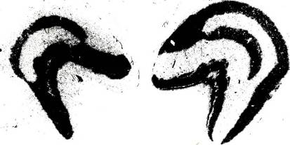
Rice. 73. In these sections of the external geniculate bodies - left and right - one can see the concentration of radioactive tracer in the three layers associated with the left eye. One week before sectioning, the left eye was injected with tritium-labeled proline. Those layers in which the mark has accumulated appear darker and thicker on the autograph.
In order to observe such a picture of the organization of the tubing, not much radioactive substance needs to be injected into the eye. If, during injection, it is administered in a sufficiently large quantity, then its concentration in the layers of the tubing will become so high that part of the radioactive label will pass from the endings of the optic nerve fibers into the cells of the tubing themselves (within the labeled layers) and will be transported along their axons to the striate cortex. As a result, the tracer will begin to accumulate in the endings in layer 4C, forming a regular pattern corresponding to the eye in which the injection was made. When the autoradiograph is ready (this requires several months, since the concentration of the labeled substance that reaches the cortex is very low), we will actually see on the cross section of the cortex where the label accumulates in layer 4C (Fig. 74). If we cut the bark parallel to its surface (by first straightening the bark or cutting it into pieces and then fastening successive sections together), then we can finally see the distribution of columns as if we were looking at the surface of the bark from above. A clearly defined set of parallel stripes can be seen both in a single slice (Fig. 75, top) and in the reconstructed image (Fig. 75, bottom). In all these autoradiographs of the cortex, labeled areas, i.e. the projections of the left eye appear light, and the unlabeled spaces between them—the projections of the right eye—look dark. Since from layer 4 the paths to the upper and lower layers go mainly in the vertical direction, straight up and down, then in three-dimensional space the ocular dominance zones form a system of alternating “slices” corresponding to the right and left eyes (Fig. 76).
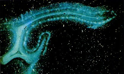
Rice. 74. On this autograph of a section of the striate cortex, the light areas correspond to those places in layer 4 where a lot of radioactive substance accumulated after its injection into the left eye of the animal. These areas are separated by dark zones that do not contain a radioactive label - zones of dominance of the right eye.
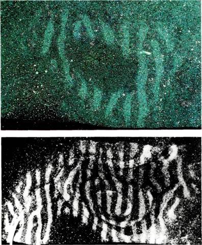
Rice. 75. Up: a section of a dome-shaped portion of the cortex running parallel to the surface of the brain. Layer 4, intersecting with the cut, forms a ring. Down: the result of combining several such rings obtained from a series of sections (the deeper the cut is made, the larger the diameter of the ring). (The picture is not very clear, since it is difficult to photograph all the sections under the same conditions, especially considering that the author is just an amateur photographer).
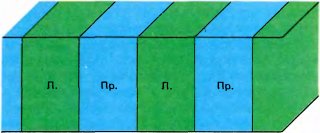
Rice. 76. In a three-dimensional representation, the columns of ocular dominance are more like not Greek columns, but like slices of sliced bread located perpendicular to the surface.
Using a different method, S. Le-Wey successfully reconstructed the appearance of the entire striate cortex in the occipital lobe. The area of the cortex lying on the surface of the brain is shown in Fig. 77. The distribution of stripes turned out to be most regular and clear at some distance from the cortical projection of the fovea. Near this projection, the pattern, for unknown reasons, is most complex - it is regular, but contains many loops and curls, so it here bears little resemblance to the regular pattern, reminiscent of a wallpaper pattern, which is characteristic of areas of the cortex more distant from the projection of the fovea. The width of the strips is constant everywhere and is approximately 0.5 mm. In percentage terms, the cortical representations of the right and left eyes are approximately equal, as long as we are talking about the projection of the central region of the retina with a diameter of about 40°. Le-Vay and D. van Essen found that beyond this region, due to a decrease in the contribution of the ipsilateral eye, the corresponding stripes narrow to 0.25 mm. If we talk about the projection of the zone 70–80° distant from the fovea, then, of course, only the ipsilateral eye is represented here. This is natural, since the field of vision of the right eye extends further to the right than to the left.
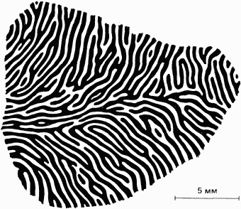
Rice. 77. Shown here is the result of reconstruction of ocular dominance zones according to Le-Vay (part of area 17 of the right hemisphere).
A second method for studying ocular dominance columns allows them to be detected throughout the entire cortex, and not just in layer 4. This is a method using labeled 2-deoxyglucose, invented in 1976 by L. Sokoloff at the National Institutes of Health in Bethesda. It is also based on the ability of radioactive substances to expose photographic film. It is based on the fact that neurons, like most other cells in the body, consume glucose as a source of energy, and the harder they have to work, the more glucose they consume. Therefore one could imagine the following procedure. The animal is injected with radioactive glucose and then one eye, such as the right eye, is stimulated by presenting a figure for several minutes (the stimulation time must be sufficient for the excited cells in the brain to absorb the injected glucose). After this, the brain is removed, sections are made and covered with photographic emulsion, and then, after proper exposure, an autoradiograph is obtained, as in the previous case. However, in reality, this scheme is not suitable, since the glucose absorbed by the cells is broken down to form products that quickly pass back into the blood. In order to prevent this leakage, Sokoloff proposed an ingenious trick - using deoxyglucose, which is very close in chemical structure to regular glucose, when injecting. “Deceived” cells absorb it and even try to break it down; however, this process is interrupted after the first step; deoxyglucose is converted to 2-deoxyglucose-6-phosphate, which cannot be broken down further. Fortunately, this substance is insoluble in the lipids of the cell membrane and therefore cannot leave the cell. It accumulates in the cell in such quantities that it can already be detected using autoradiography. By examining the result of this procedure—autograph—one can get an idea of which areas of the brain were most active during the stimulation period and accumulated the most of this “fake glucose.” If during the experiment the animal made movements with its paw, then the corresponding part of the motor cortex would also be revealed on the radioautograph. What we see after stimulation of the right eye is that part of the cortex that was most excited by this stimulus, namely a set of ocular dominance columns for the right eye. Examples of the results obtained are presented in Fig. 78.
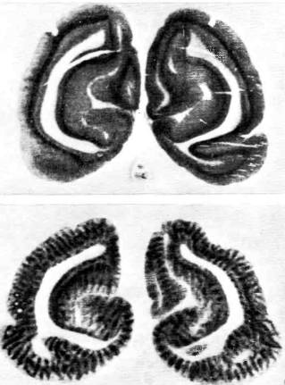
Rice. 78. Results of two experiments with radioactive deoxyglucose. Up: a slice passing through the occipital lobes of both hemispheres of an animal that perceived visual stimuli with both eyes after intravenous administration of a tracer. Down: After the injection, the animal perceived the stimulus with only one eye (the other was closed). In this case, ocular dominance columns are clearly visible in the cortex. (Experiments by C. Kennedy, M. N. Des Rosiers, O. Sakurada, M. Shinohara, M. Reivich, T. W. Tehle, L. Sokoloff.)
The idea of the same research method was successfully developed by R. Tootell from the laboratory of Russell de Valois at Berkeley, taking as a stimulus for an animal looking at a screen with one eye a large figure in the form of concentric circles and radial lines (Fig. 79, top). The resulting picture of the cortical projection also contained circles and radii, but only in a distorted form, which is associated with the unequal increase in different parts of the retina in their projection onto the striate cortex (this is also associated with the difference in visual acuity in the periphery of the retina and in the fovea). In addition, each of the circles and each of the radii are divided into many small sections corresponding to ocular dominance columns. If both eyes were stimulated simultaneously, the stripes would be continuous. It rarely happens that in one experiment it is possible to demonstrate so clearly several important facts at once.
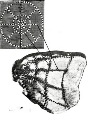
Rice. 79. In this experiment, conducted by R. Tootell, a stimulus resembling a target with several radial lines was presented in the center of the visual field of an anesthetized macaque monkey for 45 minutes. Previously, the animal was given an injection of radioactive 2-deoxyglucose. One eye was closed. The lower part of the figure shows the distribution of the label in the striate cortex of the left hemisphere of the brain. This autoradiograph shows a section of the cortex parallel to its surface. Before cutting, the cortical tissue was stretched and frozen. Semicircular lines of the stimulus are displayed in the cortex as almost vertical lines, and radial lines of the right part of the visual field are displayed as horizontal lines. The “dotted” nature of each line on the radioautograph is due to the fact that only one eye was stimulated in the experiment and, therefore, only the corresponding ocular dominance columns were excited.
Columns of ocular dominance are found in cats, some lower apes, chimpanzees and humans. Rodents and tupaya do not have them. Among the Saimiri (a genus of New World monkeys), some indications of the possible existence of such columns were obtained in physiological experiments, but modern methods of morphological analysis do not reveal them. We currently do not know the role of this complex distribution of signals coming from different eyes; it is possible that it has something to do with stereoscopic vision.
Division into areas with functionally specialized cells was found not only in the striate cortex. Such areas were first described in the mid-1960s by V. Mountcastle in the somatosensory cortex. This was the most important discovery since the first information about the localization of brain functions was obtained. The somatosensory cortex has the same relationship to touch and proprioception as the striate cortex has to vision. Mountcastle showed that this region is divided into vertically oriented zones, within which cells are sensitive to touch, and zones, in which cells respond to joint flexion or the application of significant pressure to the limb. As in the case of ocular dominance columns, the width of these zones is approximately 0.5 mm. However, it is not yet clear whether these zones form stripes, a checkerboard pattern, or individual islands against a general background. Mountcastle named them columns, and one might think that he mentally imagined some kind of honeycomb-like structure. We now know that a more appropriate term for the visual cortex would be plate or slab. However, the terminology introduced is very difficult to change, so it is probably best to keep the old term, despite its shortcomings. Today we are talking about columnar organization, when some property of the cells remains constant throughout the entire thickness of the cortex from its surface to the white matter, but changes in directions parallel to the surface of the cortex. For reasons that will become clear in the next chapter, we do not usually use this term when talking about topographic mapping, i.e. about the projection of the location of receptive fields on the retina or on the surface of the body.
Orientation columns
When recording the reactions of neurons in the striate cortex, we already noticed at the very beginning that whenever the activity of two cells is simultaneously assigned, these cells turn out to be similar not only in ocular dominance, but also in the optimal orientation of the stimulus. The question arises: are neighboring cells of the same type in all other properties? The answer will be no. As I have already mentioned, the positions of the receptive fields do not coincide exactly in most cases, although the fields usually overlap; directional sensitivity is often opposite, or in one cell it may be well expressed, while in another it may not be present at all. In layers 2 and 3, where cells that respond to the ends of lines meet, one cell may not exhibit this property at all, while the neighboring one may have it fully. On the other hand, it is very rare for two adjacent cells to show a clear difference in optimal stimulus orientation or opposite ocular dominance.
The preferred orientation, as well as ocular dominance, remains unchanged when the electrode passes vertically through the entire thickness of the cortex. As already mentioned, in layer 4C? cells generally have no selectivity for stimulus orientation; but as soon as we reach layer 5, the cells show a strongly pronounced tuning to a certain orientation, and the optimal orientation here is the same as it was above layer 4. If we now remove the electrode and insert it in some other place, then the overall picture will remain the same, only the orientation will most likely be different. Thus, the cortex is divided into narrow regions with a constant preferred orientation that extend from the surface of the cortex to the white matter, but are interrupted in layer 4, where the cells have no orientation selectivity.
If, on the contrary, the electrode is inserted parallel to the surface of the cortex, then a surprisingly regular change in the preferred orientation is observed - each time the electrode is moved 0.05 mm (50 μm), the orientation shifts on average 10° clockwise or counterclockwise. Therefore, when the electrode moves 1 mm, it usually changes to the opposite. The values of 50 µm and 10° are close to the limit of currently available measurement accuracy, so it is impossible to say definitively whether the orientation changes continuously when the electrode is displaced or shifts intermittently.
In Fig. 80 and 81 show part of a typical experiment in which the electrode was advanced into field 17 in a direction close to horizontal. In this experiment, the fixation points of the two eyes on the screen did not completely coincide (due to anesthesia and the injection of a substance that relaxes the muscles) - the distance between them was about 2°. Colored circles in Fig. 86 approximately correspond to the size of the receptive fields (about 1° in diameter), located 4° below and to the left of the central fovea (responses from cells in the right hemisphere were recorded). The first cell, labeled 96, was binocular, but the next, 114, was clearly dominated by the right eye. Then there are cells numbered from 111 to 118 with dominance of the left eye. It is easy to see how the orientation in a sequence of cells changes regularly, in this case in a counterclockwise direction. If you plot the dependence of orientation on electrode advancement (Fig. 87), then all points will fall on a line close to a straight line. The transition from one eye to the other was not accompanied by any sudden changes in either the direction of the orientation shift or the slope of the line on the graph. According to our interpretation, this means that there is no close connection between the two grouping systems—by ocular dominance and by stimulus orientation. It looks as if the cortex were marked in two completely independent ways.
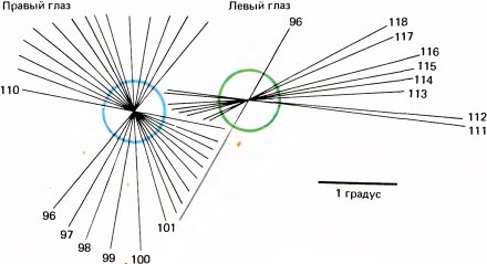
Rice. 80. If a microelectrode is inserted very obliquely into field 17 of the macaque cortex, a very regular change in orientation selectivity is detected (in this case, 23 neighboring cells were studied).
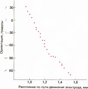
Rice. 81. Graphical representation of the results shown in Fig. 80. This is a plot of optimal stimulus orientation (in angular degrees) versus the distance traveled by the microelectrode. (Since the electrode was inserted almost parallel to the cortical surface, the penetration length is almost the same as the corresponding distance on the cortical surface). In this experiment, a complete 180° rotation of the stimulus orientation occurred over a path of 0.7 mm.
As the electrode is advanced parallel to the cortical surface, the optimal stimulus orientation may change either clockwise or counterclockwise. In most cases, if the electrode path is long enough, the direction of the orientation shift will sooner or later reverse. The moment of such a change, or reversion, is unpredictable, but it usually occurs at intervals of several millimeters. In Fig. 82 shows an example of such successive changes in direction.
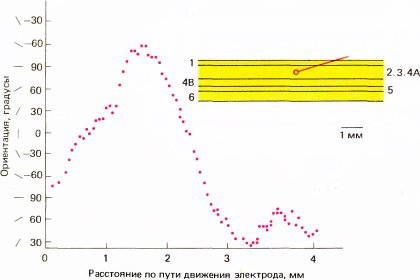
Rice. 82. The results of another experiment, presented in the form of a graph of the optimal orientation of the stimulus versus the distance traveled by the electrode. Three reversal points are visible, in the intervals between which direct proportionality is maintained.
Finally, in some experiments we discovered another feature, which we called rupture Just when we were beginning to be hypnotized by the monotonous regularity of a gradual change in orientation in the same direction, this course of events was suddenly - in rare cases - interrupted, and an orientation shift immediately occurred by 45-90°. After this, the same regular sequence continued again, only its direction was often reversed. In Fig. 83 shows an example of such discontinuities located at a distance of several tenths of a millimeter from each other.
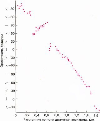
Rice. 83. The case of the appearance of two discontinuities, i.e. points at which the optimal orientation suddenly changes. Before and after these points there is a smooth change in the optimal orientation.
What would areas of constant orientation look like when looking at the cortex from above? This question turned out to be much more difficult to answer than a similar question about ocular dominance columns. Until very recently, we did not have a direct opportunity to “see” orientation groups and could only try to logically deduce their shape from the results of microelectrode studies such as those described above. The presence of both reversions and discontinuities suggests the complexity of the configuration of interest to us. On the other hand, the linear regularity that we observed frequently millimeter by millimeter along the cortex may indicate periodicity, at least within small zones of the cortex; then reversions and discontinuities might indicate that this periodicity is interrupted every few millimeters.
In those areas where periodicity is preserved, it is possible to reconstruct the desired configuration with a certain probability. Let us assume that this configuration is such that within this region, when moving the electrode parallel to the surface of the cortex, we observe periodicity without reversals and breaks, i.e. Everywhere we get a graph like in Fig. 81. If we had a sufficient number of such graphs, we could reconstruct the three-dimensional structure (Fig. 84); here is the vertical axis (z) displays the orientation, and the horizontal axes (x и y) — distances in the plane of the cortex. In this case, the orientations would be displayed on some surface; for example, if the graph is a straight line, then this surface would look like an inclined plane, as shown in Fig. 84, and in other cases it would be a curved surface. In such three-dimensional reconstructions, the desired surfaces would be intersected by horizontal planes (the plane x — y or planes parallel to it) along some lines corresponding to a constant orientation (these lines can be called iso-orientational), which is similar to isohypses on geographical maps. Uneven terrain - hills, depressions, mountains - in such a three-dimensional reconstruction will give in some areas reversals in the graphs of orientation versus distance, and sharp changes in elevation in the form of steep cliffs will lead to discontinuities. The main conclusion from these arguments is that the presence of regularity zones means that it is possible to construct a map with isolines, which means that areas of constant orientation, when viewed from above, should have the appearance of stripes. Since the preferred orientations remain unchanged during vertical penetration of the crust, in a three-dimensional representation these areas should have the appearance of plates. And since the iso-orientation lines can be curved, these plates will not necessarily be regularly shaped bodies, like evenly cut slices of bread. Much of the above has been demonstrated in direct experiments in which two or three penetrations were made in parallel directions at a distance of no more than a millimeter from each other. The result of these experiments was the reconstruction of a three-dimensional picture at least within the small area studied.
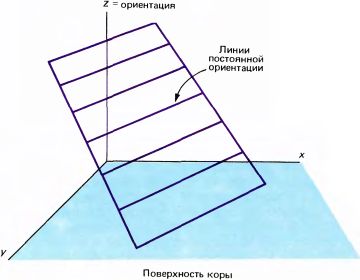
Rice. 84. Three-dimensional representation where the surface of the cortex is located in a plane x-y, and the optimal stimulus orientation is plotted along the vertical axis z. If all directions of electrode motion produce a linear relationship between orientation and distance, then the resulting surface will be a plane and will intersect the plane x-y (if the surface is not flat, it will still intersect with this plane). In this case, when drawing planes parallel to the plane x-y, isolines will be obtained. (This statement looks at first glance more complicated than it actually is! The same can be reasoned if the plane x-y will be the surface of Tierra del Fuego, and along the axis z will be plotted by elevation, average January precipitation, or temperature.)
If our reasoning is correct, then when performing many arbitrary penetrations, some of them will coincidentally coincide with the direction of the orientation contours, and then the orientation should remain unchanged. This does happen, but not very often. This was to be expected, since trigonometry dictates that even a small deviation in the direction of penetration from the contour line should lead to quite large changes in orientation; therefore, only in very few cases can graphs of orientation versus electrode insertion depth turn out to be horizontal lines.
The number of orientation gradations represented in one square millimeter of cortex can be determined from the steepest graphs obtained in the experiment. This figure is approximately 400 degrees per 1 mm, which implies that the full range of orientations within 180 degrees can be contained in an area of about 0.5 mm in length. This value will need to be remembered when we return to the question of the topography of the crust and its amazing homogeneity. However, looking ahead, I would like to note that the thickness of a pair of ocular dominance columns is approximately 0.4 + 0.4 mm, i.e. close to 1 mm. This is twice the thickness of a complete set of orientation plates, but the order of magnitude is the same.
Soon, however, we used the deoxyglucose mapping method, which allowed us to directly study the geometry of the orientation columns. To do this, we simply took as a stimulus a drawing of parallel stripes with a constant orientation, say vertical, which was presented throughout the entire experiment. The resulting picture (Fig. 85) turned out to be much more complex than the picture of ocular dominance columns. However, even here the regularity of the distribution was clearly visible with a period of 1 mm or slightly less (the distance from the middle of one dark stripe to the middle of the next). This is consistent with electrophysiological data (with the distance by which the electrode must be moved from cells with a certain orientation, say vertical, in order to reach the vertical orientation again through all intermediate options). In some places we found a structure in the form of regular stripes over an area of several square millimeters. We wondered: is there some connection between the configurations of the orientation stripes and ocular dominance stripes - maybe, for example, they run parallel or intersect at right angles? In the same experiment, we were able to identify ocular-dominant columns after a radioactive amino acid was injected into the animal's eye, and then the resulting tissue sections were analyzed using two techniques (the result is shown in Fig. 86). We were unable to detect any clear correlation. Comparing the complex pattern of orientation columns with the much simpler distribution of ocular dominance columns, it was very difficult to decide which could be a connection between them.
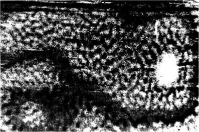
Rice. 85. After an injection of deoxyglucose, an anesthetized monkey was presented with a stimulus in the form of slowly moving black and white stripes. In the resulting autoradiography one can see a periodic distribution of the mark, in particular in layers 5 and 6 (a large area to the left of the center). The round spot located even further to the left is due to the uniform distribution of the mark and corresponds to layer 4C?; this is to be expected since cells in this layer are insensitive to orientation.
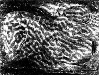
Rice. 86. The same animal as in the previous case had a radioactive amino acid (proline) injected into its eye a week earlier. After washing the section in water to dissolve 2-deoxyglucose, autoradiography was obtained. The radioactive label reveals ocular dominance columns here. These columns have no visible connection with the orientation columns.
The method using deoxyglucose has one serious drawback: there is never complete confidence that the resulting distribution pattern is actually related to the property of the stimulus that interests us. For example, when a pattern of black and white vertical stripes is used as a stimulus, how can one be sure that the resulting distribution is related precisely to the orientation of these stripes, i.e. that in the dark areas there are cells that respond to vertical lines, and in the light areas there are cells that do not respond to them? Instead, the decisive feature of a given stimulus might be that it is black and white and not color, or that it consists of wide rather than narrow stripes, or, finally, that the screen is located precisely at this rather than another distance from the animal. One indirect evidence that the action of deoxyglucose affects orientation tuning mechanisms is the absence of any spots or stripes in layer 4C, where cells do not have orientation selectivity. Another confirmation is the result obtained in the research of M. Stryker from the University of California at San Francisco. Stryker made extended penetrations with a microelectrode in the striate cortex of cats parallel to its surface and each time he encountered cells with a certain optimal orientation, he produced local destruction of the tissue; then, after injection of radioactive deoxyglucose, a stimulus with stripes of the same orientation was turned on. In these experiments, a clear correlation was found between the resulting label distribution on the histological section and the orientation of the stimulus.
Orientation columns have recently been most clearly identified using voltage-sensitive dyes, which were developed over many years by L. Cohen at Yale. G. Blasdel from the University of Pittsburgh used them in studying the cerebral cortex. In this method, a voltage-sensitive dye that stains cell membranes is applied to the surface of the cortex of an anesthetized animal, and the nerve cells absorb it. When an animal is presented with a stimulus in an experiment, all cells that respond to it change their color. If there are enough such cells in an area close to the surface of the cortex, these color changes can be captured using modern methods of processing television images. Although color changes are subtle, sensitive cameras and machine noise filtering techniques can detect them. Blasdel used stimulation in his experiments with stripes of a certain orientation, after which he photographed the resulting distribution of cell activity over an area of several square centimeters. The same procedure was then repeated for many other stimulus orientations. After this, each orientation was assigned its own color - red for vertical, orange for the clockwise position at 1 o'clock, etc.; then all the images were superimposed on each other. Because the iso-orientation line must gradually shift as the orientation changes, a rainbow pattern should appear in any small area of the image. This is what Blasdel actually found. There are still few examples of successful application of this method, and there is no way to interpret the resulting images in terms of discontinuities and reversals, but the method seems promising.
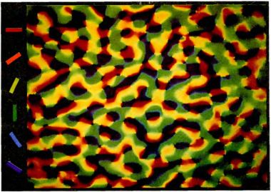
Rice. 87. In this experiment, G. Blasdel used voltage-sensitive staining to treat the monkey striate cortex. The monkey was presented with strips of sequentially changing orientation. The image of the cortex was obtained using television technology. Using computer image processing, a final image was obtained in which the areas that responded to a particular stimulus orientation were assigned a specific color. In any small area of the cortex, orientation zones appear as parallel stripes, so that as a whole, a complete set of elements tuned to different orientations gives a picture painted in all the colors of the rainbow.
Cortex maps
Now that we have learned something about the topographic representation in the cortex of orientation and ocular dominance parameters, we can consider the relationship between these mappings and projections of visual fields. It is usually said that the retina maps to the cortex in a one-to-one fashion. However, given what we know about the receptive fields of cortical cells, it is safe to say that this statement is not strictly speaking true, since each cell receives input from thousands of rods and cones, and its receptive field is far from a point. The mapping from the retina to the cortex is much more complex than any ordinary one-to-one mapping. In Fig. 88 I have tried to show the distribution in the cortex of those areas that are activated by a simple stimulus (this should not be confused with the receptive field of a single neuron). The stimulus here is a short segment of a line with an inclination of 60° relative to the vertical, presented only to the left eye. We hypothesize that this element of the visual field projects to the cortical region outlined by the rounded rectangle. Within this region, only those bands that are associated with the left eye will be excited, and within these bands, only those areas that correspond to the 60° orientation. All of them are blackened out in the picture. Thus, the line that appears in the field of view causes a bizarre picture of the distribution of excited cortical cells in the form of a series of narrow stripes.
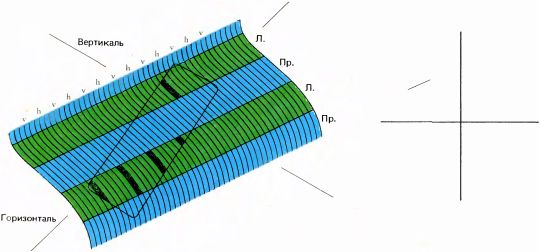
Rice. 88. An inclined line segment presented to the left eye (right) could cause a distribution of excitation in a small area of the striate cortex shown on the left. The excited areas will be limited to a small area of the cortex - long and narrow in accordance with the shape of the stimulus. Within this zone itself, excitation is limited to the ocular dominance columns for the left eye and only to those orientation columns that correspond to the clockwise orientation at 2.00 or 8.00. As you can see, the cortical mapping of this stimulus is not so simple!
Now it becomes clear how naive the idea of a green homunculus, which sits in our heads and examines the picture transmitted to the cortex, is. In fact, the picture that is created in the cortex has approximately the same relation to the image of the external world as the electrical processes in a television camera have to do with the transmitted external scene. If the distribution of cortical activity exactly reproduced the distribution of brightness in the visual field, then this would mean that nothing significant happened on the way from the retina to the cortex. In this case, a little green man would really be needed.
It is hardly possible to imagine that so much effort in the process of evolution would have been spent on such an elegant grouping of cells in two mutually independent systems of columns if this did not provide some benefit to the animal. Until we get to the bottom of the precise wiring that determines the mapping of the retina into the cortex, we are unlikely to fully understand the principles of cell grouping in the cortex. Right now we can only make logical guesses. If we assume that the diagram given in Chapter 4 corresponds to reality, then we will have to admit that what is needed to move from simple cells to complex ones, or to create sensitivity to the ends of lines or to the direction of movement, is a certain kind of convergence of many cells onto one cell, and the receptive fields of the intermediate cells must have the same orientation and approximately the same position. So far we have had no particular reason to assume that a cell with a certain orientation of the receptive field receives inputs from cells with receptive fields of a different orientation. (I am exaggerating somewhat here: it has been suggested that cells with different optimal orientations of stimuli may be connected by inhibitory connections; there is only indirect evidence in favor of this, in my opinion, not very convincing, although it cannot be ignored.) If this is so, then why not group together cells that should be mutually connected? The alternative is hardly practical - it is easy to imagine how difficult it would be to ensure proper connections between cells if these cells are scattered throughout the cortex without taking into account their similar properties! There should be especially many connections between cells with the same optimal orientation, and if such cells were distributed randomly, the network of axons necessary to connect them would fill all the space between neurons. Be that as it may, they are actually grouped together. The above considerations also apply to cells similar in ocular dominance.
But if cells with similar properties pack together, why do we see successive changes in orientation in small steps as we advance the electrode? And what explains the cyclicality - why, having gone through all possible options, we again return to the original orientation, and then the whole cycle repeats again? It would seem that one could collect together all the cells with an orientation of 30°, all the cells with an orientation of 42°, etc.; and finally, combine all cells with dominance of the left eye and all with dominance of the right eye. If we knew how the cortex works, we could offer many answers to these questions. Now we will make one assumption: it is possible that cells with different orientations actually have an inhibitory effect on each other. If it is undesirable for a cell to respond to orientations other than its own, then it is not difficult to imagine the presence of inhibitory connections that sharpen the tuning of a given cell to a particular orientation. Then the observed picture is exactly what we need: cells with the same orientation are located closest to each other, but not too far from cells with a different, but very similar orientation; then the inhibitory connections will be quite short. Another possibility is that if we consider what inputs from cells in layer 4 (with round fields) are needed to organize a simple cell with a certain optimal orientation, it is easy to see that only a small change in the set of inputs will be required in order to obtain a closely spaced simple cell with a similar but slightly different orientation. To do this, it is enough to add several new inputs and remove several old ones (Fig. 89). Considerations of this kind would explain the physical proximity of cells with similar orientations.
The subject of the next chapter will be the relationship between orientation, ocular dominance, and the projection of the visual field onto the cortex. Considering this question may help us understand why so many columns are needed. When the question of topography is added to this, the corresponding cortical organization will appear even more complex and interesting.
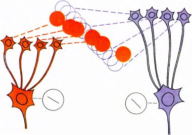
Rice. 89. Shown is a group of layer 4 cells with concentric receptive fields needed to create a simple cell responding to a slant line with the orientation "4.00 - 10.00". Probably, this group has common cells with the group necessary to react to a line with the orientation “4.30 - 10.30” - to transform one group into another, it is enough to remove a few connections and add a few.
\n
Eye, brain, vision\n
\nDavid Hunter Hubel; David Hunter Hubel;