Primary visual cortex
After Kuffler's first paper on the receptive fields of retinal ganglion cells with a center and periphery was published in 1952, avenues for further work opened up. To explain the discovered properties of these cells, additional research was needed at the retinal level. However, data about the next levels of the visual system was also required to understand how the brain interprets the information provided by the eyes. Solving these two problems was fraught with enormous difficulties. When studying the central mechanisms, it took several years to develop a method for long-term (on the order of several hours) recording of the activity of a single cell. It was even more difficult to select visual stimuli that influenced this activity.
Topographic mapping
Before it became possible to continue work in this direction, there was already some information about the areas of the brain associated with visual function: the initial stages of the transmission of visual information were fairly well traced (Fig. 35). We knew that optic nerve fibers synapse with cells of the lateral geniculate body (UCC) and that the axons of GC cells terminate in the primary visual cortex. It was also clear that these connections - from the retina to the NKT and from the NKT to the cortex - have topographic organization. Speaking of topographic mapping, we mean that the previous structure is projected onto the subsequent one in an orderly manner: if you go along any line on the retina, then the projections of successive points of this line in the NKT and in the cortex also form one continuous line. Thus, the fibers of the optic nerve emerging from a small area of the retina will all be directed to some small area of the NKT, and all fibers from a small area of the NKT will come to a certain area of the visual cortex. This organization of connections will not seem surprising if we recall the simplified diagram of the nervous system in Fig. 13: The cells here are grouped into a structure resembling a stack of plates, with each cell in any plate receiving inputs from some compact group of cells in the previous plate.
In the retina, successive layers of cells are arranged like playing cards in a deck, so that nerve fibers can take shortcuts from one layer to the next. The cells of the external geniculate bodies are located at some distance from the cells of the retina, just as the cortex is distant from the NKT and is located in a different part of the brain. However, the nature of the connections between cells remains the same - the projections of individual zones to higher levels are organized as if these zones were exactly superimposed on each other.
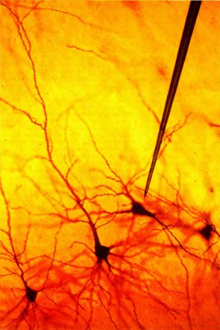
Rice. 34. In the visual cortex of the monkey, Golgi staining reveals only a few pyramidal cells - a tiny fraction of the total number in the section. In reality, the height of the rectangular section shown here is about a millimeter. Superimposed on the microphotograph is an image (at the same scale) of a typical tungsten electrode used in extracellular recording of neuronal activity.
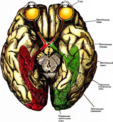
Rice. 35. Visual pathways in the human brain, from the eyes to the primary visual cortex (ventral view). Let the input image fall on those halves of both retinas that are colored red here (these are their right halves, since the brain is upside down). The opposite half of space (left visual field) is projected onto these areas; Ultimately, the input information is transmitted to the right half of the brain (the paths of its transmission are also colored red). This occurs because approximately half of the fibers that form the optic nerve pass to the other side at the chiasm, while the other half remains on the same side. Thus, firstly, each hemisphere receives information from both eyes; secondly, each hemisphere receives information about the opposite half of the visible world.
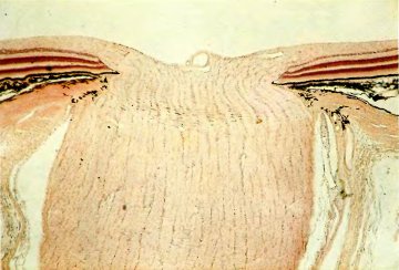
Rice. 36. The optic nerve where it exits the eye, interrupting the layers of the retina shown on the left and right. The width of the area shown in the micrograph is about 2 mm. The free zone at the top of the picture is the internal environment of the eye. The section shows the layers of the retina (from top to bottom): optic nerve fibers (light), three colored layers of cells and a black layer containing the melanin pigment.
At the exit from the eyeball, the optic nerve fibers simply gather into a bundle. Having reached the tubing, they diverge and form a topographically ordered projection with their ends. (The surprising thing is that in the optic nerve, on the way from the retina to the NKT, these fibers are almost completely mixed up, but in the NKT they again “find their places.”) In the same way, the fibers emerging from the NKT diverge in the form of a wide strip that goes through the entire brain to the back of the head and ends in the primary visual cortex, where the projection again appears ordered. After these pathways, having passed through the primary visual cortex and formed synapses in its various layers, leave this area and reach other cortical zones, they again form a topographically ordered projection. As convergence of connections occurs at each level, the receptive fields as a whole gradually become closer, so the further away from the retina, the more blurry the visually perceived picture will be.
Another important and long-standing evidence in favor of the topographic organization of the visual pathways comes from clinical observations. If a certain area of the primary visual cortex is damaged, “local blindness” develops, as if the corresponding area of the retina had been destroyed.
So, the visual world is systematically reflected in the structures of the external geniculate bodies and the cortex. However, in the 50s it was unclear what such a display might mean. At that time, it was not yet obvious that the brain processes the information it receives, transforming it into a form that is more convenient for use. It was believed that the visual scene is simply transmitted to the brain, and its task is to comprehend it (or this task, perhaps, is solved not by the brain at all, but by the mind). In subsequent chapters we will learn that a neural structure such as the primary visual cortex produces profound transformations of incoming information. We know almost nothing about what happens at further stages of its processing. Therefore, one could say that we have not progressed very far. However, the knowledge that a certain part of the cortex uses completely understandable principles in its work gives grounds for optimism - it allows us to assume that other areas of the cortex work the same way. Perhaps the day will come when we won't have to use the word "mind" at all.
Cell responses in the lateral geniculate body
Fibers traveling to the brain from each eye pass through the optic chiasm (from the name of the Greek letter “chi” - ?). At the chiasm, approximately half of the fibers of each optic nerve travel to the opposite side of the brain to that eye, while the other half remain on the same side of the brain. After passing through the chiasm, the fibers are directed to several different points. Some of them go to neural structures related to such specific reactions as eye movements and the pupillary reflex. However, most of the fibers terminate in the two external geniculate bodies (ECBs). Compared to the cortex and many other parts of the brain, these bodies are relatively simple in structure - all or almost all of the approximately one and a half million cells in each NKT have direct inputs from optic nerve fibers, and most cells (but not all) send their axons to the cerebral cortex. It follows that the pathways passing through the NKT into the cortex have only one synaptic switch. However, it would be a mistake to consider tubing as simply a transfer station. This includes not only fibers from the optic nerve, but also fibers coming back from those areas of the cortex to which the NKTs are projected, as well as from the reticular formation of the brain stem, which is related to the processes of attention and general activation (arousal). Some NKT cells have short axons (less than a millimeter in length); they do not extend beyond the NKT, but form synaptic contacts with other NKT neurons. Despite these complications, single NKT cells respond to light stimuli in much the same way as retinal ganglion cells, and they have similar on- and off-center receptive field structures and similar responses to color stimuli. Thus, when it comes to processing visual information, NCT does not appear to produce any significant signal transformations. As for the nonvisual inputs of the NKT and local synaptic connections, so far we simply do not know anything about their role.
Representation of right and left sides in the visual pathway
The optic nerve fibers are distributed between the two tubing in an unusual and, at first glance, even strange way. Fibers from the left half of the retina of the left eye go to the NKT of the same side of the brain, while fibers from the left half of the retina of the right eye pass in the chiasma to the other side and thus enter the same left NKT (this is shown in Fig. 35). Similarly, fibers from the right halves of both retinas also end in one - the right - hemisphere. Because the lens creates an inverted image on the retina, light rays emanating from the right half of the visual scene are projected onto the left halves of both retinas and information is transmitted to the left hemisphere.
The term visual fields Those areas of the surrounding world or visual scene that are visible with both eyes are designated. Right visual field includes all points lying to the right of the vertical passing through the point that we fix with our gaze (Fig. 37). It is important to distinguish visual fields, those. what we see in the outside world, from receptive field, which corresponds to that part of the external world that a single cell “sees”. To paraphrase what was said at the beginning of this section, we can say that information from the right half of the visual field is transferred to the left hemisphere.
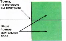
Rice. 37. The right visual field extends to the right almost 90°. You can easily verify this if you quickly bend and straighten your finger and slowly move it in a circle to the right. Upward the field of view extends 60° or so, downward about 75°, and to the left, by definition, extends to the vertical, passing through the point at which you fix your gaze.
Many other parts of the brain are structured in a similar way. For example, tactile and pain signals from the right side of the body come to the left hemisphere, and motor control of the muscles on the right side of the body is carried out by the left hemisphere. A massive stroke to the left side of the brain results in paralysis and loss of sensation in the right side of the face, right leg and right arm, as well as loss of speech. But, what is less known, such a stroke is usually accompanied by loss of vision in the right half of the visual field, and for both eye. To establish the presence of such blindness, the neurologist asks the patient to stand in front of him, close one eye and look with the other at the tip of the doctor’s nose. Then he begins to examine the patient’s visual fields, moving his hand or a special probe to different points in space. In the case of a left-sided stroke, it can be shown that the patient does not see anything to the right of the fixation point. For example, if a doctor raises a probe in his hand and holds it between himself and the patient a little above his head, then when the hand moves slowly from right to left (from the patient’s point of view), the patient does not see anything until the white sleeve of the doctor’s coat crosses the midline and suddenly appears in the patient’s field of vision. If you check the other eye, the result will be exactly the same. Complete right-sided homonymous hemianopsia (this is what neurologists call such loss of half of the visual field!) will also accurately divide the area of the fovea (center of gaze): if you look at the word was, fixing your gaze on the middle of the letter A, then the letters will not be visible s, and even from the letter а only its left half will remain - an interesting, but very upsetting experience.
These kinds of tests clearly show that signals from each eye are transmitted to both hemispheres and that, conversely, each hemisphere of the brain receives input signals from both eyes. This may seem strange: after what has been said about the sense of touch, pain and the motor control system, the reader may assume that the left eye should send signals to the right hemisphere and vice versa. However, in the case of the visual system, each hemisphere of the brain deals not with the opposite side of the body, but with the opposite half surrounding space. But, however, the situation when signals from the left eye are transmitted mostly to the right hemisphere (and vice versa), occurs in many lower mammals, such as horses and mice, and even in birds and amphibians complete crossing of the optic nerves. In horses and mice, the eyes are positioned so that they point laterally rather than straight ahead, resulting in most of the retina of the right eye displaying the right visual field, whereas in primates the eyes are directed straight ahead and there are displays of both the right and left visual fields on each retina. The above description of the visual pathways applies only to those mammals whose eyes look more or less straight (as, for example, primates) and therefore see almost the same area of the surrounding world.
The auditory system is structured in a similar way. It is clear that each ear is capable of hearing sounds emanating from both the left and right halves of the surrounding space. Like the eyes, each ear transmits sound information approximately equally to both sides of the brain. Moreover, in the auditory system, as in the visual system, the process of information transmission is lateralized: the sound reaching each ear from a certain source on the right side is analyzed in the brain stem by comparing the amplitudes and moments of arrival of signals to both ears, and as a result, the reaction to this sound is formed mainly in the higher parts of the left half of the brain.
Here we are talking about the initial stages of information processing. If there is a person standing to my right who, with words or gestures, encourages me to do something with my left hand, then the information he communicates must sooner or later get into the right hemisphere of my brain. However, the signals must initially arrive in the auditory or visual cortex of the left hemisphere, and only after that they are transmitted to the motor cortex of the right hemisphere.
By the way, no one knows Why the right half of the surrounding space is usually projected into the left hemisphere of the brain. There is one important exception to this rule - the cerebellar hemispheres (the part of the brain that primarily controls movement) receive input signals primarily from the same, rather than the opposite, side of the surrounding space. This complicates the functioning of the brain because all the fibers connecting one hemisphere of the cerebellum to the motor cortex in the other hemisphere of the cerebrum must travel from one side of the brain to the other. All that can be said about such an organization for now is that it seems mysterious.
Layered structure of the external geniculate body (ECB)
Each tubing contains six cell layers. A separate layer is several cells thick (from 4 to 10 or more). This entire six-layer sandwich is bent in such a way that its cross section has the appearance shown in Fig. 38.
When moving from the retina to the NKT, a simple scheme in which each subsequent layer of cells contains a projection of the previous one becomes more complex. In NKT, projections from the retinas of the two eyes are combined, and two separate images, represented at the level of ganglion cells in the retinas, are projected onto the six layers of NKT. Fibers from the right and left eyes do not converge on the same cells of the NKT - each of these cells receives signals only from one eye. The two sets of cells are separated into separate layers, so that in any given layer, all cells receive information from only one eye. These layers are arranged in such a way that projections from the right and left eyes alternate. Thus, in the left tubing the projections are arranged in the following order (from the surface to the depth): left, right, left, right, right, left. It's not entirely clear why the sequence of layers 5 and 6 is "reversed" (sometimes I think it's done to make the order of the projections harder to remember). We do not yet have any intelligible explanation for the very fact of alternation of projections.
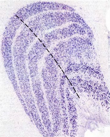
Rice. 38. Left lateral geniculate body of the macaque. Six cell layers are clearly visible. The cut is made parallel to the frontal plane; it is specially colored to reveal the cell bodies of neurons (each one looks like a dot).
In general, the six-layer neural structure has one common topography for all layers. The left halves of both retinas are projected into the layers of the left NKT (Fig. 39), and the right halves are projected into the layers of the right NKT. Any point in one layer of tubing corresponds to a certain point in the field of view of one or the other eye. If you move along the tubing layer, then the corresponding point in the field of view will move along a certain trajectory determined by the nature of the display of the visual field on the tubing. If we move perpendicular to the layers of the tubing (for example, along the black dashed line in Fig. 38), as a microelectrode would move when passing through different layers, then the corresponding receptive fields of the cells would remain in the same part of the visual field; in this case, only an alternation of projections from different eyes would be observed, with the exception, of course, of the place where two projections from one eye occur in a row. Thus, each half of the field of view is displayed six times on each of the tubing, three times for each eye, and the projections in the layers of the tubing are located exactly below each other.
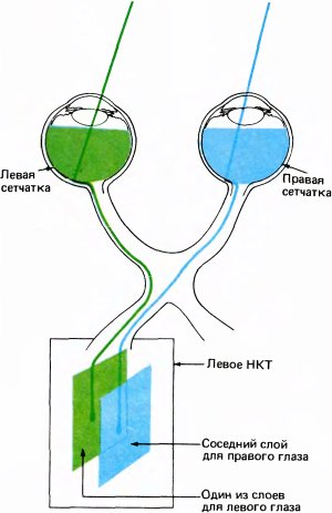
Rice. 39. During the transition from the retina to the NKT, the spatial ordering of neurons is preserved, although along this path it temporarily disappears when the fibers gather into a bundle; in the CNT they again “find their places.”
The lateral geniculate body appears to be composed of two parts. It is divided into ventral, or lower, layers and four dorsal, or upper, layers (ventral - located closer to the ventral side of the body, dorsal - to the dorsal side). The ventral part of the NKT forms a special structure, since the cells in the corresponding layers differ from the cells in the other four layers - they are larger and respond differently to visual stimuli. At the same time, the four layers of the dorsal part of the NKT are similar to each other both histologically and in their electrophysiological properties. Since the size of the cells in these two sections is different, the ventral layers began to be called large cell, and the dorsal ones - small cell.
The fibers emerging from the six layers of tubing are combined into one wide bundle called visual radiation, which goes up to the primary visual cortex (see Fig. 35). Here, these fibers diverge evenly and are redistributed so that a complete projection with a topographic organization is formed (this is similar to the distribution of the fibers of the optic nerve as it enters the NKT). And now, finally, we come to the bark.
Cell responses in the cortex
The main theme of this chapter is the question of how cells in the primary visual cortex respond to visual stimuli. The receptive fields of NKT neurons have the same organization (division into center and periphery) as the receptive fields of retinal ganglion cells, which send their axons to NKT cells. Like retinal ganglion cells, NKT neurons differ from each other mainly in the properties of the receptive field (on- or off-center, location in the visual field) and the characteristics of responses to color stimuli. The question arises: what about cortical neurons? Are they similar to NKT cells that send their axons to the cortex, or do they have some new features? The answer, as the reader should already have guessed, is that cortical cells do indeed have new properties, so unusual that until 1958, when they first began to be studied using complex light stimuli, no one could even approximately predict these properties.
The primary visual cortex (striate cortex) is a layer of cells 2 mm thick and several square inches in area.[1] In order to give an idea of the size of this neural structure, the following figures can be cited: if the NKT contains one and a half million cells, then the striate cortex contains about 200 million cells. The anatomical structure of the striate cortex is surprisingly complex, but it is not necessary to know its details in order to understand how incoming visual information is transformed here. The structure of this department will be discussed in more detail in the next chapter, where the issue of its functional architecture will be discussed.
As I already said, the process of processing information in the cortex consists of several stages. At the first stage, most cells give the same responses as NKT cells. The receptive fields of these cells have circular symmetry. This means that a line or boundary (difference in illumination) produces the same response regardless of its orientation. It is not easy to record the electrical activity of cortical cells at this level, since they are very small and located close to each other. It is not yet clear whether the responses of these cortical cells differ at all from those of NKT cells (just as it is not clear whether the responses of NKT cells differ from those of retinal ganglion cells). The complexity of the histological structure of the NKT and the cortex suggests that there must be some differences between them and that they can be identified if you know where to look for them; however, this may be difficult to know.
The situation becomes even more complicated when we move to the responses of cells at the next cortical level. Probably, these cells should receive input signals from neurons of the previous level, which have receptive fields with a center and a periphery. At first, it was not at all easy for us to figure out what visual stimuli these cells of the second cortical level responded to. At that time (late 50s), very few researchers attempted to record the responses of single neurons in the visual cortex. Those who have done this have had conflicting results. They found that cells in the visual cortex appear to work in much the same way as those in the retina—both on- and off-cells were found. In addition, another class of cells was discovered that did not seem to respond to light stimuli at all. The simplicity of the identified physiological properties of cortical cells against the background of the simply diabolical complexity of the morphology of the cortex baffled researchers.
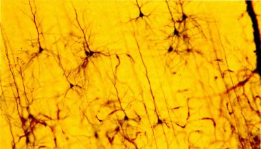
Rice. 40. Golgi-stained section of the primary visual cortex, showing more than a dozen pyramidal cells (but this is only a very small fraction of the neurons contained in the section). The vertical size of the depicted area is about 1 mm. (The dark stripe at the right edge is a blood vessel.)
Today it is very easy to explain. Firstly, inadequate stimuli were used - to activate cortical cells, out of habit, they simply illuminated the entire retina with scattered light, although Kuffler had shown ten years earlier that such stimulation even for retinal neurons was far from optimal. For the majority of cortical neurons, diffuse illumination of the retina is not only not optimal, but generally a completely ineffective stimulus. If many cells of the external geniculate bodies still respond, albeit weakly, to diffuse illumination, then cortical cells, even those belonging to the first cortical level and similar to the cells of the NKT, practically do not respond to such stimulation. Thus, the first thought that came to mind, that to activate visual neurons it is best to stimulate all the receptors in the retina, turned out to be completely wrong. Secondly (and this is even more paradoxical), it turned out that those cortical cells that gave on- or off-responses were in fact not cells, but simply axons of NKT cells. The actual cortical neurons in this case did not respond to stimulation at all! They considered it beneath their dignity to pay attention to such a primitive stimulus as diffuse light.
This was exactly the case in 1958, when Torsten Wiesel and I managed to carry out one of the first successful taps of electrical activity from the cortex in a cat. In these experiments, the position of the microelectrode tip in the cortical tissue was so stable that it was possible to listen to the activity of the same cell for about nine hours. To cause cell discharges, we used all possible and impossible means - except that we ourselves did not stand on our heads. (Like most cortical cells, from time to time the found cell would fire spontaneously, but we tried to convince each other that the discharge was caused by our stimuli, and as a result we wasted a lot of time.) After several hours of unsuccessful attempts, we had the vague impression that applying light to one specific area of the retina caused some reaction, and we concentrated our efforts on that area. We mainly used round white and black spots as stimuli. To create a black spot, we usually took a glass slide measuring 2.5 x 5 cm, onto which an opaque circle was glued; the glass was inserted into a special projection device that Samuel Talbot designed to project images onto the retina. To present white spots, we took a copper plate of the same size with a small hole (in those days the cost of conducting research was much lower). After about five hours of hard work, it suddenly seemed to us that when, from time to time, the cell randomly gave a reaction, the reaction was probably not due to the black speck applied to the glass, but to the glass itself. In the end, we were able to establish that the cell's reaction was caused by a weak but clear shadow from the edge of the glass plate when it was pushed into the window of the projection device. We soon became convinced that this edge worked as a stimulus only when its shadow crossed a certain area of the retina, and this shadow had to have a very specific orientation. The most surprising thing was the sharp difference in the results in two cases - when the orientation of the stimulus was optimal (then the discharge resembled a machine gun fire) and when we changed the orientation of the stimulus or completely illuminated the eye with a bright flash (in this case there was no reaction).
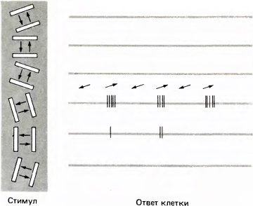
Rice. 41. Responses from one of the first orientation-sensitive cells that Torsten Wiesel and I discovered in the cat striate cortex in 1958. This cell responded exclusively to a stimulus in the form of a moving slit with an orientation corresponding to the clockwise position at 11 o'clock; at the same time, she responded to the upward movement of the stimulus to the right and did not respond to the downward movement to the left.
This phenomenon was discovered first and sent us down the wrong path. The fact is that, as luck would have it, the discovered cell type was exactly the one that we later called the class complex cells, and they belong to a level two steps higher than the first cortical level of cells with receptive fields divided into center and periphery. Although complex cells are the most common cell type in the striate cortex, their properties are difficult to understand without first becoming familiar with the cells of the previous, intermediate level.
Indeed, in contrast to the cells of the first level, which have receptive fields with a center and periphery, in the monkey, cells of higher levels show completely different reactions. Typically, point light stimuli elicit only weak responses from these cells or are not effective at all. In order to evoke a cell response, you first need to find the appropriate area of the visual field to present the stimulus, i.e. find the corresponding section of the screen in front of which the animal is located. In other words, we must first identify the receptive field of a given cell. After this, it turns out that the most effective stimulus for a given cell is a line moving in the receptive field in a direction perpendicular to the orientation of the line. This line could be a narrow strip of light on a dark background (slit), a dark stripe on a light background, or a straight line between dark and light areas. Some cells showed a preference, often a very strong one, for one of these three stimuli, while others responded with approximately equal intensity to all three types of stimuli. The orientation of the line was of decisive importance - most often, the cell responded best to a certain optimal orientation, and the intensity of the response (the number of impulses that occurred when the stimulus crossed the receptive field) decreased noticeably when the orientation deviated in any direction from the optimal by 10–20 degrees; with an even greater deviation, the reaction dropped sharply to zero (see Fig. 41). The indicated figure of 10–20 degrees may seem very approximate. Remember, however, that the difference in the position of the hour hand showing “one” and “two” is even greater - 30 degrees. When the orientation of a stimulus differs by 90 degrees from the optimal orientation, a typical orientation-selective cell stops responding altogether.
In contrast to cells at lower levels of the visual system, neurons selectively sensitive to stimulus orientation respond much better to moving lines than to stationary lines. That is why (see Fig. 41) when stimulating such neurons we used lines moving through the receptive field. If a stationary, flashing (periodically flashing) line is used as a stimulus, the cell often gives a weak response, in which case the same orientation is preferred as with a moving line.
Many cells (probably a third of the entire population) make another characteristic type of response to a moving stimulus. Instead of firing the same impulse regardless of the direction of movement, such cells respond more vigorously in one specific direction. It even happens that movement in one direction causes a strongly pronounced response, and when moving in the opposite direction there is no reaction at all (this is shown in Fig. 41).
In one experiment, the reactions of 200–300 cells can be assessed if, after a complete study of one cell, the microelectrode is simply moved further to the next cell. The disadvantage of this technique is that in one run you can only study cells lying in the cortex in one straight line: once you have inserted the thinnest microelectrode into the cortical tissue, you can no longer move it in the transverse direction without damaging the electrode itself or even more delicate nervous tissue. With this recording technique, the most we can do is examine approximately 50 cells per millimeter with one microelectrode pass. When we examine the orientation selectivity of several hundred or thousands of cells, it turns out that all stimulus orientations occur approximately equally often—vertical, horizontal, and all the oblique orientations in between. If we consider the characteristic features of the world around us, which includes both trees and the horizon, the question arises: are there any distinguished orientations, such as vertical and horizontal, that are more common than others? When trying to answer this question in different laboratories, slightly different results were obtained. However, all researchers agree that if such preferences do exist, they must be very small - so small that statistical processing of the data is required to detect them. And in this case they hardly have any meaning!
In the striate cortex of monkeys, approximately 70–80% of cells have orientation selectivity properties. In cats, all cortical cells appear to be sensitive to stimulus orientation, even those that have direct input from the lateral geniculate body.
We found marked differences among orientation-specific cells, not so much in the optimal orientation of the stimulus or in the position of the receptive field on the retina, but in the nature of the behavior of the cells. The most significant difference between the two classes of neurons is simple и complex cells. As their names suggest, cells of these two classes differ in the complexity of their responses. Therefore, we made a natural assumption that cells with simpler behavior are located in the neural structure of the cortex closer to its input.
Simple cells
In most cases, the responses of simple cells to a stimulus in the form of a small spot of light can predict their response to a stimulus of a complex shape. Each of the simple cells, like retinal ganglion cells, NKT cells, and cortical cells with centrally symmetric receptive fields, has a small, well-defined receptive field. The presentation of a stimulus in the form of a spot of light within this receptive field causes either an on- or off-reaction, depending on which part of the receptive field the stimulus is presented to. The difference between simple cells and cells of previous levels lies in the configuration of the zones of excitation and inhibition. At the previous levels, this is a centrally symmetrical configuration - there is one central on- or off-zone (exciting or inhibitory) and a ring zone surrounding it on all sides with opposite properties (inhibitory or excitatory). Simple cortical cells are more complex. The zones of excitation and inhibition in their receptive fields are always separated by one straight line or two parallel lines (Fig. 42). The most common configuration is when a long and narrow excitatory zone is adjoined on both sides by wider inhibitory zones (Fig. 42, А).
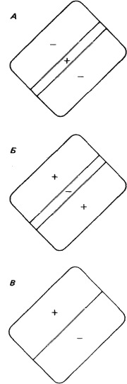
Rice. 42. Maps of three typical receptive fields of simple cells. The optimal stimuli were: for the cell А - light stripe opposite the exciting area (+); for the cage Б - dark line covering the braking zone (–); for the cage В - a sharp “dark-light” boundary, coinciding with the boundary between the excitatory and inhibitory zones.
In order to test the putative receptive field map generated by small spot testing, we tried other stimulus configurations. We soon found out that the greater the proportion of a particular zone of the receptive field covered by a given stimulus, the more pronounced the cell’s excitation or inhibition. In other words, there is spatial summation local impacts. We also discovered the phenomenon antagonism — mutual cancellation of local influences with simultaneous stimulation of the excitatory and inhibitory zones. Thus, for a cell with the receptive field shown in Fig. 42, A, the most suitable stimulus would be in the form of a narrow strip located in the receptive field so that it exactly coincides with the excitatory zone and does not enter the inhibitory zone (see Fig. 43). Even a slight change in the orientation of this band will lead to a decrease in the effective area of the excitation zone and will also affect the inhibitory zone; as a result, the firing rate of the cell's response will decrease.
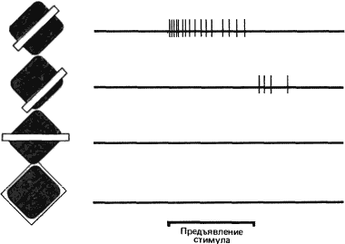
Rice. 43. Stimuli of different configurations cause different reactions of a cell with a receptive field of the same type as А in Fig. 42. The thick line segment at the bottom indicates the period (1 second) when the stimulus was turned on - the light stripe. The first case (top entry) shows the cell's response to a strip of optimal size, position and orientation. In the second case, the same stripe covers only part of the inhibitory zone (since this cell does not have spontaneous activity that could be suppressed during inhibition, here only the discharge of the cell is visible when the stimulus is turned off). In the third case, the stripe is oriented so that it covers only a small part of the excitatory zone and, accordingly, a small part of the inhibitory zone, and therefore the cell does not respond at all. The bottom entry shows the case of uniform illumination of the entire receptive field: there is no answer here either.
In Fig. 42, Б и В the receptive fields of simple cells of the other two types are shown, which respond best to dark lines and to rectilinear boundaries of light and dark; At the same time, the sensitivity of cells to stimulus orientation remains approximately the same as in cells of the first type. Cells of all three types do not respond at all to the stimulus of diffuse illumination. This mutual cancellation of the processes of excitation and inhibition is reminiscent of the reaction of neutralization of an acid with a base, which students perform in laboratory work in chemistry. Thus, already at this cortical level there is a large variety of neurons. If we take the class of simple cells, then they have three or four different types of receptive fields, and there are cells tuned to any of the possible orientations of the stimulus, and cells with a receptive field in any part of the visual field.
The size of the receptive fields of simple cells depends on their distance from the fovea. However, in the same area of the retina there are also some differences in the size of the receptive fields. The smallest receptive fields, located in and near the fovea, have a value of approximately 0.25–0.25°. As for the cells of the type shown in Fig. 42, А и B, then the width of the central zone is no more than a few arc minutes. This value coincides with the minimum diameter of the receptive fields of retinal ganglion cells or NKT cells. If we take the region of the distant periphery, then the size of the receptive fields of simple cells here can reach 1?1°.
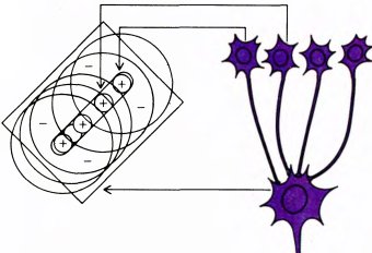
Rice. 44. Possible diagram of connections that determine the receptive field of a simple cell. Four cells form excitatory synaptic connections with a higher order cell. Each of the lower-order cells has a receptive field with radial symmetry, an excitatory center and an inhibitory periphery (this is shown in the diagram on the left). The centers of these receptive fields lie along a straight line. If we assume that a given simple cell is connected to many cells that have receptive fields with a center and a periphery, and the centers of these receptive fields overlap and lie on the same straight line, then the receptive field of a simple cell will consist of a long, narrow excitatory zone and inhibitory flanks. Avoiding technical terminology, we can simply say that a small bright spot anywhere in this long and narrow rectangle will lead to strong excitation of one or more cells with circular receptive fields and as a result activate, albeit weakly, a simple cell. If the stimulus is a long narrow strip capable of activating all cells with round receptive fields, then this will lead to a strong response of a simple cell
Even now, twenty years later, we still do not know how the input circuits for cortical cells are arranged, on which the specific reactions of these cells depend. A number of plausible schemes have been proposed, and it may well turn out that one of these schemes, or some combination of them, turns out to be correct. The properties of simple cells can be determined by upstream neurons with circular receptive fields; The easiest way is to assume that simple cells have direct excitatory inputs from many cells of the previous level - those whose centers of receptive fields lie in the visual field on the same straight line (Fig. 44).
It is somewhat more difficult to propose a hypothetical scheme for cells that selectively respond to the boundaries of dark and light (see Fig. 42, В). The following option is possible: this simple cell has inputs from two sets of cells of the previous level, in which the centers of the receptive fields are located on two sides of the same line - on one side of the cell with on-centers, and on the other with off-centers, and all these inputs are excitatory. In all such hypothetical schemes, the excitatory input from an on-center cell is logically equivalent to the inhibitory input from an off-center cell, provided that the off-center cell has spontaneous activity.
Finding out the actual mechanism that determines the reactions of simple cells is not an easy task. Regarding a given simple cell, it will be necessary to find out from what kind of cells it receives input signals, for example, to find out for each of the preceding cells the structure of the receptive field, its location and orientation (if any), the type of center (on- or off-), as well as the nature of the signals sent - whether they are excitatory or inhibitory. Since there are no methods for obtaining such information yet, we are forced to use indirect approaches, and this increases the likelihood of error. The diagram shown in Fig. 44 seems to me the most plausible, since it is the simplest.
Complex cells
Complex cells correspond to the next level (or levels) of visual analysis. They are most numerous in the striate cortex and constitute here probably about three-quarters of the entire population of neurons. The first orientation-sensitive cell that Wiesel and I studied—the one that responded to the edge of a glass slide—was almost certainly a complex cell.
A common property of complex and simple cells is the ability to respond only to lines oriented in a certain way. Complex cells, like simple ones, respond to stimuli presented in a limited area of the visual field. They differ from simple ones in that their reactions cannot be explained by the shape and distribution of excitatory and inhibitory zones in the receptive field. Turning on or off a small stationary spot within the receptive field rarely causes the cell to respond. Even to a properly oriented stationary stripe or boundary, the cell most often does not respond or gives only a weak, quickly decaying response of the same type both when the stimulus is turned on and when the stimulus is turned off. However, if a properly oriented line is moved across the receptive field, a well-defined, sustained discharge of impulses occurs. This discharge begins the moment the line enters the receptive field and continues until it leaves its limits (see Fig. 41, which shows the response diagram). On the contrary, in order to cause a long-term discharge of a simple cell, it is necessary to present a properly oriented stationary line in a certain part of the receptive field. If you use a moving line, then only a short-term reaction occurs at the moment when the line crosses the border of the inhibitory and excitatory zones, or at the time when the line passes through the excitatory zone of the receptive field. Those complex cells that are capable of responding to stationary light “slits”, stripes or boundaries, produce a pulsed discharge regardless of where in the receptive field the stimulus is located, as long as its orientation is appropriate. However, the same stimuli are completely ineffective if their orientation is far from optimal (Fig. 46).

Rice. 45. The activity of this cell from layer 5 of the cat striate cortex was recorded in 1973 using an intracellular electrode by D. Essen and J. Kelly of Harvard Medical School. Her complex receptive field was also mapped. Then, by injecting the dye procion yellow, they found out that it was a pyramidal cell.
Schemes in Fig. 46 (for a complex cell) and in Fig. 43 (for a simple cell) demonstrate a significant difference between the two types of cells: in a simple cell, a reaction is caused by an optimally oriented line only in a very narrow range of positions, while in a complex cell such a line causes a response, no matter in which part of the receptive field it is presented. This difference is due to the existence of clearly defined excitatory and inhibitory zones in the receptive field of a simple cell and their absence in the receptive field of a complex cell. A complex cell provides an example of the generalization (nonlocality) of a response to a line within a larger region.
In general, complex cells have slightly larger receptive fields than simple cells, but not by much. In macaques, in the area of the fovea, receptive fields of complex cells with a size of approximately 0.5–0.5° are most often found. In this region of the retina, the optimal stimulus size for both simple and complex cells is about two arcminutes. Thus, the “resolution power” of complex cells is the same as that of simple cells.
As with simple cells, we do not really know how the communication system that transmits signals to complex cells is organized. However, here too it is not difficult to propose several possible schemes for their organization. In the simplest of these schemes, a complex cell receives input from many simple cells whose receptive fields have the same orientation but are distributed, partially overlapping, across the entire field of the complex cell, as shown in Fig. 47. If connections from simple cells to complex cells are excitatory, then whenever a stimulus in the form of a line enters the receptive field of a complex cell, they are excited some simple cells. As a result, the complex cell will also be excited.
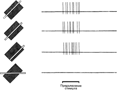
Rice. 46. A long and narrow strip of light causes a reaction in a complex cell regardless of where in the receptive field it is presented, as long as its orientation is optimal (top three entries). If the orientation of the stripe differs from the optimal one, the cell responds weaker or does not respond at all (bottom entry).
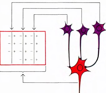
Rice. 47. A diagram of connections that would explain the observed properties of a complex cell. We assume that (as in Fig. 44) one complex cell can receive excitatory signals from a large number of simple cells (only three are shown here). Each simple cell responds best to the vertical boundary between light (left) and dark (right) regions. It is assumed that the receptive fields of simple cells are scattered within the rectangle and overlap. If a stimulus in the form of such a boundary is applied to any place in the rectangle, then a certain number of simple cells are activated and this in turn causes a response from a complex cell. Due to the synaptic adaptation effect, only a moving stimulus will cause continuous excitation of the complex cell.
Typically, in response to a stationary line, the complex cell fires a short burst (even if the stimulus remains on). In this case we say what is happening adaptation answer. If you move a line in the receptive field of a complex cell, a continuous discharge is observed: adaptation is overcome as a result of the sequential firing of new simple cells.
The reader must have noticed that both of the above connection diagrams—from cells with round receptive fields to simple cells (Fig. 44) and from simple cells to complex cells (Fig. 47)—suggest the use of excitatory connections. However, in these two cases the excitation processes must be completely different. The first of these schemes requires summation simultaneous signals from cells with round receptive fields lying on the same line. In the second scheme, to activate a complex cell by a moving stimulus, it is necessary sequential excitation of many simple cells. It would be interesting to find out what morphological differences (if any) this difference in the summation mechanism is associated with.
Directional selectivity
Many complex cells respond better to a stimulus moving in one direction than in the opposite direction. The difference in reaction is often very sharp - with one direction of movement an energetic response occurs, and with the opposite direction the cell does not respond at all (Fig. 48). As it turned out, approximately 10–20% of cells in the upper layers of the striate cortex exhibit noticeable directional selectivity. The remaining cells do not seem to have such selectivity - we carefully examined the responses of the cells using a computer, trying to detect even a small difference in responses to the movement of a stimulus in opposite directions. Thus, there appear to be two different classes of cells—one of them clearly exhibits directional selectivity, while the other does not.
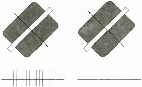
Rice. 48. The reactions of a given complex cell to the movement of an optimally oriented strip in opposite directions are different. The duration of each recording is about 2 seconds. (For such cells, it doesn't particularly matter how fast the stripe is moving; usually the cell will not respond only when the movement is very fast, in which the stripe appears blurred, or when it is so slow that it is difficult to notice at all.)
If you listen to the impulse response of a cell with strongly pronounced directional selectivity, you get the impression that when a line moves in one direction, the stimulus seems to sharply push the cell and causes it to discharge, and when moving in the opposite direction, a malfunction occurs and the stimulus becomes ineffective (this is reminiscent of the situation when, while winding a watch, you turn the head of the winding mechanism back and a characteristic crack is heard).
We do not know how the input networks of such cells with directional selectivity are structured. It is possible that simple cells are connected to the input of such a cell, the reactions of which to the movement of a stimulus in opposite directions are unequal and asymmetrical. The receptive fields of such simple cells are asymmetrical, such as, for example, the field shown in Fig. 42, IN. Another possible scheme was proposed in 1965 by G. Barlow and W. Levick to explain the directional selectivity of some cells in the rabbit retina - cells that apparently do not exist in the monkey. If we apply their scheme to complex cells of the cortex, then we must assume the presence of an intermediate layer of cells located between simple and complex cells (as in Fig. 49). Let us imagine that a cell from the intermediate layer has an excitatory input from one simple cell and an inhibitory input from another cell, the receptive field of which is directly adjacent to the previous one, and, moreover, always on the same side. Let us further assume that the inhibitory path includes some delay, perhaps due to the inclusion of another intermediate cell. In this case, if the stimulus moves in one direction, say from right to left (as in Fig. 49, illustrating the model of Barlow and Levick), then the intermediate cell is excited by a signal from one of its inputs just at the moment when inhibition comes from another cell, the receptive field of which the stimulus has just crossed. The excitatory and inhibitory effects neutralize each other, and as a result the cell does not produce an impulse discharge. If the stimulus moves in the opposite direction, inhibition occurs too late to prevent the impulse discharge. If many such intermediate cells converge on some cell located at the next, third, level, then this cell will have the properties of a complex cell with directional selectivity.
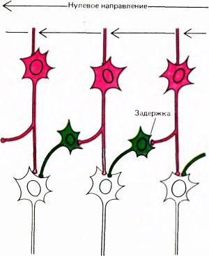
Rice. 49. This scheme was proposed by H. Barlow and W. Levick to explain the properties of directional sensitivity. Synapses that red cells form on green cells are excitatory, and synapses formed on white cells are inhibitory. We assume that three white cells (bottom) converge onto one “master” cell.
We do not have direct evidence of the correctness of certain hierarchical schemes that explain the observed cell reactions, i.e. schemes in which cells at each subsequent level are organized on the basis of elements of the previous level. Nevertheless, we have good reason to believe that the nervous system is organized according to a hierarchical principle. One of the most serious reasons for this conclusion is related to morphology - for example, in cats, simple cells are concentrated in the fourth layer of the striate cortex, i.e. in the layer that receives inputs from the cells of the lateral geniculate bodies, while complex cells are located in the layers of the cortex above and below - one or two synaptic switches further from the input. Thus, although we cannot provide an exact pattern of connections at each level, we have good reason to believe that such a pattern exists.
The main reason that in complex cells we see the result of a certain organization of cells with round receptive fields with a center and a periphery is the obvious need to process information logically in two stages. I would like to emphasize the word logically, since, in general, the required transformation, apparently, could be physically carried out in one stage - if we sum up the input signals from cells with round receptive fields on the individual branches of the dendrites of complex cells. In this case, each branch would perform the functions of a separate simple cell, sending signals to the cell body (and therefore to the axon) electrotonically (using a passive electrical process) whenever any line falls into a certain zone of the corresponding receptive field. In this case, such a cell itself would exhibit the properties of a complex cell. However, the very presence of simple cells makes us think that we should not build such complex imaginary structures.
The Importance of Motion Sensing Cells (including some comments on how we "see")
Why are there so many motion-sensitive cells? First of all, it comes to mind that such cells signal whether there is a moving object in the field of view. For animals, including you and me, changes in the external world are much more important than confirmation of its immutability, whether we are talking about the survival of a predator or prey. It is therefore not surprising that most cortical cells respond better to moving objects. Following this logic, you must now question how we then analyze stationary visual scenes when, in the interests of motion sensitivity, so many cells tuned to a particular stimulus orientation are insensitive to stationary contours. To answer this question, we need to backtrack a bit and look at some important but counterintuitive evidence about how we “see.”
First of all, it would be natural to expect that when examining the world around us, our eyes would smoothly scan the entire scene with continuous movements. In fact, when fixating an object, this is what happens: first, we position our eyes so that the image of this object falls in the area of the central fovea of both eyes, then we hold our eyes in this position for a short time, say half a second, then the eyes abruptly move to a new position and fixate a new target, which is located somewhere else in the visual field and attracts attention by the fact that it moves slightly relative to the background or has some interesting shape. During such a jump, or saccades, the speed of eye movement is so high that the visual system does not have time to react to the movement of the image across the retina and we simply do not notice it. (It is possible that, in a sense, vision is turned off for the period of the jump by some complex neural circuit that connects the oculomotor centers with the main visual pathway.) Thus, the process of examining the visual field when reading or simply viewing the surrounding space consists of a series of rapid jumps from one point to another.
Special recording of eye movements allows us to clearly demonstrate how invisible these jumps are to us. To record eye movements, they take a tiny mirror and attach it to the side of the contact lens so that it does not interfere with vision. After this, a beam of light is directed onto the mirror, which, when reflected, creates a small spot of light on the screen. There is another way to record eye movements, a more modern one; it was developed by D. Robinson at the Wilmer Institute (Johns Hopkins University). In this technique, a tiny inductor coil is mounted on the edge of the contact lens on the subject's eye, and the subject is placed between two mutually perpendicular hoops the size of a bicycle wheel, on which other inductance coils are located. The flow of current in these coils leads to the appearance of current in the coil on the contact lens. Once such a system is calibrated, eye movements can be recorded with great accuracy. For the poor subject himself, neither one nor the other method of recording eye movements can be called pleasant!
In 1957, Soviet psychophysicist A.L. Yarbus recorded the eye movements of subjects while viewing various images, in particular such as a scene in the forest and a woman's face (Fig. 50). In these recordings, periods of gaze fixation are represented by dots, and the dots are connected by lines showing the trajectory of eye movement during saccades. Even a quick glance at these amazing recordings provides a lot of information about the work of our visual system - even about what objects and details of the world around us are most interesting to us.
So, the first fact that contradicts our intuition is that during visual inspection the eyes jump from one point of interest to another and that it is impossible to examine a stationary scene with smooth eye movements. The task of the oculomotor system, apparently, is not to keep the image on the retina motionless, but to prevent its smooth displacement. If the entire visual scene is moving, as happens when we look out of a train window, then we follow this scene, fixing with our gaze some object and maintaining its fixation by smooth eye movement until the object leaves the visual zone, after which we make a leap and fixate a new object. This sequence of eye movements - a smooth tracking movement, say to the right, and then a saccade to the left - is called nystagmus. You will be able to see this kind of movement yourself when you find yourself on a train or tram: watch the eye movements of your fellow passengers as they look through the window at the surrounding landscape (just be careful that your attention is not misinterpreted!). The control of eye jumps when viewing interesting elements of the scene in order to transfer their images to the fovea is carried out from the superior colliculi. This was shown in 1978 in a series of impressive works by P. Schiller from the Massachusetts Institute of Technology.
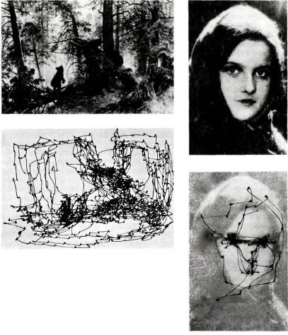
Rice. 50. The subject examines the picture, and at this time the position of his eyes and, consequently, the direction of his gaze are constantly recorded. The eyes make a jump and immediately stop (at this moment a small dot appears in the recording), then a jump follows to a new interesting place. It seems that it is difficult for the eye to jump to those parts of the picture where there are no sharp changes in brightness.
The second group of facts regarding how we see is even more contrary to our subjective impression. When we look at a stationary scene and our gaze fixes some point that attracts attention, then this fixation is not absolutely stationary. Despite all our attempts to rigidly fix the point, the eyes do not remain completely at rest, but make continuous micro-movements called microsaccades. They occur several times per second and are directed more or less randomly, reaching an amplitude of 1–2 arcminutes. In 1952, L. Riggs and F. Ratliff from Brown University and R. Ditchburn and B. Ginsborg from the University of Reading simultaneously and independently discovered that if the image on the retina is artificially stabilized (by special methods), eliminating its displacement relative to the retina, then the visual image after about a second “fades” and the field of view becomes completely empty! (The simplest method of stabilization is to attach a point light source to a contact lens; when the eyes move, the light source also moves and the light spot quickly becomes invisible.) If, after stabilization, the image on the retina is moved even slightly, the light spot immediately appears again. Apparently, microsaccades are necessary to continuously see stationary objects. It is as if Nature, when creating the visual system, was especially concerned about the perception of movement and therefore tried to ensure that cells were insensitive to stationary objects, but then she had to invent microsaccades in order to make stationary objects visible.
It can be assumed that this process involves complex cortical cells that are particularly sensitive to the movement of the stimulus, but probably does not involve cells with directional selectivity, since microsaccades are apparently randomly distributed across directions. On the other hand, the mechanism of directional selectivity would presumably be useful for detecting the movements of objects relative to a stationary background, signaling the presence of movement and its direction. In order to follow a moving object against a stationary background, you need to fixate the object and move your gaze along with it. In this case, the image of everything else will move across the retina (this situation is rare in other cases). The movement of all the details of a motionless background across the retina should lead to vigorous activity of cortical cells.
Line ends as visual stimuli
Another type of cell is found in the striate cortex. Typically, simple and complex cells are characterized by spatial summation—the longer the stimulus line, the better the response. However, the response intensifies only until the length of the line reaches the size of the receptive field: further lengthening of the line does not lead to a more energetic response. In contrast, in cells that respond to ends of lines (end stopped cells), extending the line to a certain limit continues to improve the response, and if the line goes beyond this limit (in one or both directions), then the response weakens (Fig. 51, Б). Some cells are what we call "end-of-line-only" cells (completely ended stopped cells) do not respond at all to the presentation of a stimulus in the form of a long line. We call the zone from which a cell response can be evoked activation zone (or excitatory zone), and zones located at one or both ends are inhibition zones (or inhibitory zones). Thus, the entire receptive field of such a cell consists of an excitatory zone and an inhibitory zone (or zones) at the edges. A stimulus of optimal orientation, activating a cell from the excitatory zone, causes maximum inhibition outside this zone (on one or both sides). This can be shown by repeatedly stimulating the excitatory zone with a line of optimal length and optimal orientation while simultaneously testing the outer zone with lines of different orientations (as shown in Fig. 52).
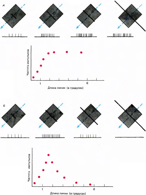
Rice. 51. A. The response of an ordinary complex cell to a light line of varying length. The duration of each recording is 2 seconds. As a graph of the response versus line length shows, the response of a given cell increases until the line reaches a length of about 2°, after which the response remains unchanged. B. For this cell responding to the ends of lines, the response increases until the line length reaches 2° and then decreases so that a line of 6° length does not produce any response.
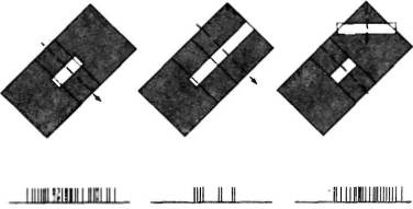
Rice. 52. For a given cell that responds to the ends of lines, presentation of one stripe with optimal orientation in the middle excitatory zone leads to the appearance of an energetic response. Involvement of one of the inhibitory zones in stimulation almost completely suppresses the cell response; however, if the stimulus has a different orientation in this inhibitory zone, the cell's initial response does not change. Thus, the optimal orientation is the same for both the excitatory zone and the inhibitory zone.
At first we thought that such cells belonged to the next level of the hierarchy of cortical neurons, a level above complex cells. According to the simplest diagram of the possible organization of such cells, they could have one or more excitatory inputs from ordinary complex cells with receptive fields located in the excitatory zone, and inhibitory inputs from complex cells with the same orientation of the receptive field, located outside the excitation zone (this diagram is explained in Fig. 53). According to another possible scheme (Fig. 54), the cell has excitatory input from cells with a small receptive field (A) and inhibitory input from cells with a large receptive field (b). It is assumed that cells that provide inhibitory signals are maximally sensitive to long lines, but are weakly excited by short lines. This second scheme (similar to the model of cells having receptive fields with a center and periphery, see page 60) is one of the few schemes that has received partial confirmation. Charles Gilbert of Rockefeller University in New York found that complex cells in layer 6 of the monkey striate cortex have exactly the properties needed for the inhibition assumed in this scheme. He also showed that if these cells were inactivated by local injections, then the cells located in the upper layers of the cortex that responded to the ends of the lines lost the ability to respond with inhibition to the ends of the lines.
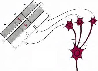
Rice. 53. One of the schemes to explain the behavior of a complex cell that responds to the ends of lines. The outputs of three ordinary complex cells converge on such a cell; in this case, in one of these cells the receptive field coincides in position with the excitatory zone of the cell that responds to the end of the stimulus (A), and in the other two cells the receptive fields lie on either side of the excitatory zone (б и в). The first cell forms an excitatory synapse at the output (+), and the other two are inhibitory synapses (–).
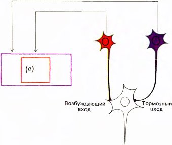
Rice. 54. An alternative scheme in which inhibition is carried out by one cell with a receptive field corresponding to the entire zone а+б+в in Fig. 53. For this scheme to work, we must assume that the inhibitory cell responds weakly to the short line when the zone is stimulated A, but responds intensely to a long line.
After the models described above were proposed, J. Henry (Canberra, Australia) discovered simple cells that respond to the end of the line, the diagram of the receptive fields of which is presented in Fig. 55. The organization scheme of such cells is similar to the first scheme proposed above, except that the inputs here are not from complex cells, but from simple ones. Thus, the responses of complex cells responding to line ends could be determined by a combination of excitatory input from one set of complex cells and inhibitory input from another set (as in the circuits shown in Figs. 53 and 54), or by the convergence of inputs from several simple cells responding to line ends.
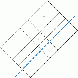
Rice. 55. It is assumed that a simple cell that responds to the ends of lines can be organized due to the convergence of input connections from three ordinary simple cells. (One of them, with an on center, could have an excitatory effect; the other two could have on centers and excitatory outputs, or off centers and inhibitory outputs.) Instead, input signals could come directly from cells with circular fields (with a center and a periphery) using a more complex version of the circuit shown in Fig. 44.
The optimal stimulus for a cell tuned to the end of a line is a line segment of a certain length. For a cell that responds to a border, and on one side responds only to its end, the ideal stimulus would be an angle; for a cell that responds to both ends of light or dark lines, the best stimulus will be a short white or black line, as well as a curved line that falls into the excitatory zone and does not fall into the inhibitory zone due to its curvature (this will happen if the orientation of its ends differs by at least 20–30° from the orientation of its middle part; a similar case is shown in Fig. 56). Thus, end-sensitive cells can be thought of as cells that are sensitive to angles, to curvature, or to sharp breaks in lines.
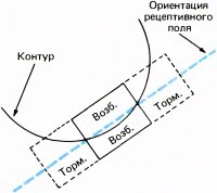
Rice. 56. For a cell that responds to the ends of lines (like the one shown in Fig. 52), a curved border can serve as an effective stimulus.
Single cell neurophysiology and visual perception
The mere fact that a brain cell responds to visual stimuli does not mean that it is directly involved in perception. For example, many neural structures in the brainstem, related primarily to the visual system, are designed only for auxiliary functions - to control eye movements or pupil constriction, to focus images using the lens. As for the cells that I described in this chapter, it is obvious that they are directly related to visual perception. As I mentioned at the beginning, the destruction of any small area of striate cortex leads to blindness in some small area of the visual field. In monkeys, damage to the striate cortex has the same effect. However, in cats the situation is more complicated - a cat with the striate cortex removed can see, although not as well as before. Other parts of the brain, such as the superior colliculus, may play a more important role in visual perception in her than in primates. Lower vertebrates such as frogs and turtles have nothing like our cerebral cortex, but no one would argue that they are blind.
We can now say with reasonable certainty what exactly any of the cortical cells described above do in response to stimulation by an image of a visible scene. Most cortical cells respond poorly to diffuse illumination and respond well to lines with the desired orientation. Thus, when presented with a figure resembling a kidney in shape (Fig. 57), this kind of cell will respond if and only if a section of the boundary with a certain orientation intersects its receptive field. The same cells whose receptive fields are located inside the boundaries of the figure will not react in any way - they will continue to give a spontaneous impulse discharge regardless of the presence or absence of this figure.
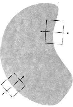
Rice. 57. How likely are the cells in our brain to respond to certain characteristic stimuli, such as the kidney-shaped figure shown here? Of the entire set of cells in the visual cortex, only a very small group of cells will respond to such a stimulus.
This is how cells with orientation selectivity behave. However, to excite a simple cell, it is not enough that the section of the contour corresponds to the optimal orientation - the contour must also almost exactly fall on the border of the inhibitory and excitatory zones of the receptive field, because for a response it is necessary that the light falls on the excitatory zone, but does not spread to the inhibitory zone. If you move a section of the contour even slightly without changing its orientation, the stimulation of this cell will be insufficient, and now another population of simple cells will begin to be excited. For complex cells, the excitation conditions are not so stringent, since the population of cells activated by a stimulus at some point in time will not change with a slight shift in the boundaries of the figure without changing their orientation. To noticeably change the population of excited complex cells, you need to move the border quite strongly - so that it completely leaves the receptive fields of some cells and enters the fields of others. Thus, the population of excited complex cells - in contrast to simple ones - generally changes little with small translational displacements of the object.
If we finally turn to the cells that respond to the ends of the lines, here too we find less stringent restrictions on the exact location of the stimulus (although each given configuration will activate many fewer cells). For neurons of this type, the orientation of the circuit must always coincide with the optimal orientation of the excitatory zone of the receptive field, but must change markedly outside this zone so that inhibition does not balance excitation. In short, a section of the circuit must have sufficient curvature or be abruptly interrupted so that all the conditions for excitation of a given cell are met (see Fig. 56).
These stringent requirements increase the selectivity of cortical reactions, since each visible object excites only a very small fraction of the cells on whose receptive fields its image falls. This specialization of cells probably continues to increase with further transition to even higher levels outside the striate cortex. Rods and cones are simply affected by light itself. Retinal ganglion cells, NKT cells and cortical neurons with the center and periphery compare the corresponding parts of the visual field with the surrounding background, so they are likely to respond to any segment of the contour that falls into their receptive field, but will not respond to a general change in retinal illumination. Cells that are selectively sensitive to orientation note not only the presence of a contour, but also its orientation and even the speed of its change, i.e. curvature of the line. If such cells are classified as complex, then they are also sensitive to movement. As discussed in an earlier section of the book, there are two possibilities regarding the role of motion sensitivity: perhaps it makes it easier to pay attention to moving objects, or perhaps this mechanism, in combination with microsaccades, supports the response of complex cells to stationary objects.
It seems to me that the boundaries between light and dark are the most important component of our visual perceptions, but, without a doubt, far from the only one. The color of different objects certainly helps in making them stand out (though it must be said that our recent work indicates that color plays a lesser role in defining shape). When visually assessing shape and depth, the distribution of light and shade on the surface of objects and the texture of their surface are also used. Although the cells we have discussed could in principle be involved in the perception of light-dark transitions and texture, they should not be expected to respond clearly to both of these features. It remains to be seen what the mechanism of texture perception is in the visual system. One possible hypothesis is that complex cells process information about halftones and textures independently, without the help of any specialized groups of cells. It is possible that such stimuli are not capable of strongly activating a large number of cells, but textures and undertones have spatial extension and could cause many cells to respond at once, although each cell would respond moderately or weakly. Perhaps the sluggish responses of many cells would be sufficient to transmit information to higher levels.
Many people, myself included, still have difficulty accepting that the interior of any figure (such as the area inside the kidney-shaped spot in Figure 57) is not a stimulus to our brain cells, and that the perception of a uniform interior field as white or black (or colored, as we will see in Chapter 8) depends only on the excitation of edge-sensitive cells. The logical argument in favor of this is the following consideration: if during the perception of the internal region, cells whose receptive fields lie within its boundaries were activated, then it should, on the contrary, be perceived as heterogeneous! Thus, if we see the entire space occupied by a figure as uniformly black, white, gray or green, then the cells with receptive fields within the boundaries of the figure have nothing to do with this. This is a hard thought to come to terms with, isn't it? However, from the point of view of an engineer constructing a machine for encoding shapes, such a mechanism would, I think, be very suitable. The only information that needs to be obtained in this case is information about the external contour of the figure; analysis of its interior becomes unnecessary. Is it any wonder that the evolution of the brain has taken a path that allows it to process information using a minimum number of cells?
When people hear about the properties of simple and complex cells, they often conclude that to fully analyze all the smallest elements of the visual field, including dark and light lines and the edges of various areas in all possible orientations, an astronomical number of cells is required. Of course it is. But the whole point is that the cortex contains an astronomical number of cells. Today we can already tell how the cells in this part of the brain work, at least how they respond to many simple visual stimuli encountered in everyday life. I suspect that no two cells in the striate cortex work exactly the same way. Indeed, whenever it was possible to simultaneously record the activity of two cells using a microelectrode, it turned out that these cells differed at least slightly from each other - in the position of the receptive fields, directional sensitivity, intensity of responses, or some other parameters. In short, it seems that if there is redundancy in this part of the brain, it is small.
Can we be sure that the described cells are actually designed specifically to detect straight line segments, and not some other stimuli? That's not to say that we and other researchers haven't tried a variety of other stimuli, including faces, world maps, and hand passes. Experience shows that it would be foolish to think that we have exhausted all possibilities. In the early 1960s, when we were satisfied with the results obtained with the cells of the striate cortex and decided to move (and in fact had already moved) to the next area, we accidentally managed to record the response of one weakly responding cell of the striate cortex. However, by making the light line shorter, we were convinced that this cell was capable of giving a very energetic reaction. That's when we stumbled upon a class of cells that respond to the ends of lines. After that, we spent almost twenty years working with monkey cortical cells before we discovered “blebs,” clusters of cells that specifically respond to color (described in Chapter 8). Having made these reservations, I must add that some of the properties found in striatal cells, such as orientation sensitivity, are undoubtedly true properties of these cells. There is much additional evidence to support this, such as the functional anatomy data described in Chapter 5.
Binocular convergence
Until now I have hardly mentioned the existence of two eyes. The question of obvious interest is: does one or another cortical cell receive input signals from both eyes, and if so, are these inputs the same in quantitative and qualitative terms?
In order to get the answer, we must return for a while to the external geniculate body (EC) and find out whether any of its cells have inputs from both eyes. NCT is the lowest level at which it would be possible to combine signals from two eyes on one cell. However, this possibility, apparently, is not realized here - two different bundles of input fibers are distributed over different cell layers, between which there is no or almost no interaction. As one might expect, given the separateness of the projections from the two eyes, a single NKT cell should respond to stimulation of one eye and not respond at all to stimulation of the other. Judging by the results of some experiments, stimuli applied to an eye that is “foreign” for a given cell of the NKT can have a weak effect on the reaction evoked from the “own” eye. However, practically we can assume that each cell is under the control of only one eye.
It is intuitively clear that the paths coming from each eye must sooner or later come together, since when we look at something, we see one complete picture. However, everyday experience tells us that if you close one eye, there will be no big change - objects will appear just as clear, just as real and just as bright. Of course, the total field of view for the two eyes will be somewhat wider, since each eye sees a larger area of \u200b\u200bspace on its side than the other eye, although this difference is only about 20-30°. A significant difference between binocular vision and monocular vision is the perception of depth, which will be discussed in Chapter 7.
In the monkey cortex, those cells that receive input from the NKT and have receptive fields with circular symmetry are similar to the NKT cells in that they are also monocular. At this cortical level, we find approximately the same number of cells excited from the left and from the right eye, at least in those areas of the cortex that serve the visual field within a radius of about 20° from the central point of fixation. However, at the next level of the cortex, binocular cells, simple and complex, are already detected, and in macaques more than half of these cells can react independently to signals from each of the eyes.
Once we have found a binocular cell, its receptive fields in both retinas can be carefully compared. First, we close the animal's right eye and map the receptive field of the cell in the left eye, noting its exact location on the screen or retina, as well as its complexity, orientation, and location of excitatory and inhibitory zones; We also find out whether the cell is simple or complex, we examine its ability to respond to the end of a line and directional sensitivity; after this, close the animal’s left eye, open the right one and repeat the entire measurement procedure from the beginning. It turned out that in the majority of binocular cells, all the properties revealed in experiments with the left eye are also detected when stimulating the right eye - the same position on the retina, the same directional sensitivity, etc. This allows us to conclude that all connections coming to a given cell from the left eye coincide in structure with connections coming from the right eye.
Speaking about such duplication of connections, one clarification needs to be made. If, having determined the optimal stimulus for a cell, its position, orientation, direction of movement, etc., we compare its responses when stimulating one eye and when stimulating the other, the intensity of the reaction will not always be the same. Some cells do fire equally well from both eyes, but others clearly fire more strongly when stimulated in a particular eye. In general, with the exception of that part of the cortical cells that serve the periphery of the visual field, we do not find any special advantage of one eye or the other - in each hemisphere the number of cells that are better activated on the opposite side (from contralateral eyes) and on the same side (from ipsilateral eyes), approximately the same. In this case, all degrees of relative dominance of the eye are encountered, ranging from cells excited exclusively from the left eye, and ending with cells responding only to stimulation of the right eye.
Now we can estimate the size of different cell populations. Let us divide all the studied cells, say 1000 of them, arbitrarily into seven classes according to the relative effectiveness of the influence of one or the other eye on them. Then we count the number of cells in each class. In Fig. Figure 58 shows the corresponding histograms for the cat and macaque. Here the similarities and differences in the distribution of cells in these animals are immediately visible. It can be seen that in both species binocular cells are found quite often, and among cells with unilateral dominance both eyes are well represented (in macaques, approximately equally), that in cats there are a lot of binocular cells, that in macaques the number of monocular and binocular cells is approximately the same, and in binocular cells the dominance of one eye is often strongly expressed (groups 2 and 5), and that the least common cells are those that are equally well activated from either eye.
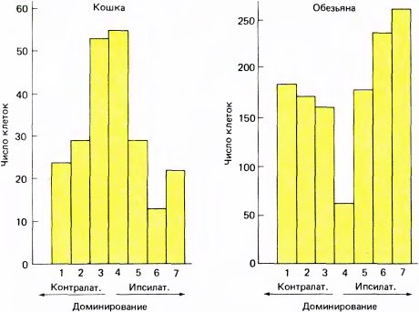
Rice. 58. Studying the distribution of neurons according to ocular dominance, we examined hundreds of cells and assigned each of them to one of seven randomly selected groups. Group 1 cells are defined as cells that are affected only by the contralateral eye, i.e. the eye located on the opposite side of the body; cells in group 2 respond to stimulation of both eyes, but clearly prefer signals from the contralateral eye; etc.
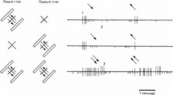
Rice. 59. The recording electrode was close enough to three cells to divert impulses from all three. The responses of different cells can be distinguished by the amplitude and shape of the impulses. The figure shows responses to stimuli presented to one eye and to both eyes. Cells 1 и 2 should be classified in group 4, since they respond almost equally to stimulation of both eyes. Cell 3 responds only to simultaneous stimulation of both eyes; all that can be said is that it does not belong to either group 1 or group 7.
We can now take this question a step further and ask: Do binocular cells respond better when both eyes are stimulated than when one eye is stimulated? It turns out that many cells are just like this - from one eye they are activated weakly or not at all, but from two eyes they give a strong impulse discharge, especially in the case when both eyes are stimulated simultaneously and in exactly the same way. In Fig. Figure 59 shows recordings of the responses of three cells (1, 2 and 3) demonstrating strong synergy. One of these cells doesn't respond at all to stimulation in just one eye, so we wouldn't be able to detect it at all unless we stimulated both eyes at the same time. The effect of synergy in many cells is weakly expressed or not observed at all - such cells respond to stimulation of both eyes in approximately the same way as to stimulation of each eye separately.
Such connections between single cells and two eyes further indicate a high degree of specificity of connections in the brain. Not only do the input connection systems of a given cell allow it to respond only to a line of a certain orientation and only to one direction of movement, it also turns out that these systems are represented by two copies, one from each eye. But this is not enough: as we learn from Chapter 9, most connections, apparently, should be formed and ready to work by the time the animal is born. All this is truly amazing.
Eye, brain, vision